=================================================================================
Scikit-learn and "sklearn" are essentially the same thing. "Scikit-learn" is the full name of the Python library, while "sklearn" is a commonly used shorthand or alias for it. The reason for this abbreviation is to make it easier and quicker to import and use the library in Python code. Scikit-learn is widely used in the machine learning community for its simplicity, ease of use, and robust implementation of various algorithms. It serves as a valuable resource for building and evaluating machine learning models across different domains with a wide range of tools for various machine learning tasks. Scikit-learn is the most popular library for modeling the types of data typically stored in DataFrames. It can be effectively used for a variety of applications, which include classification, regression, clustering, model selection, naive Bayes, grade boosting, K-means, and preprocessing. Scikit-learn requires Python (>= 2.7 or >= 3.3), NumPy (>= 1.8.2), and SciPy (>= 0.13.3) for operation. In the ML field, Spotify uses Scikit-learn for its music recommendations, and Evernote utilizes it for building their classifiers. Scikit-learn includes modules for classification, regression, clustering, dimensionality reduction, and more. Some of the algorithms and techniques available in scikit-learn include:
-
Classification Algorithms:
Support Vector Machines (SVM)
Decision Trees
Random Forests
k-Nearest Neighbors (k-NN)
Naive Bayes
Regression Algorithms:
Linear Regression
Ridge Regression
Lasso Regression
Support Vector Regression
Clustering Algorithms:
K-Means
Hierarchical clustering
Dimensionality Reduction:
Principal Component Analysis (PCA)
t-Distributed Stochastic Neighbor Embedding (t-SNE)
Ensemble Methods:
Bagging and Boosting techniques
Voting Classifiers
Preprocessing Tools:
Data scaling and normalization
Feature extraction and selection
Model Selection and Evaluation:
Cross-validation
Grid search for hyperparameter tuning
Model evaluation metrics
Neural Network Models:
Multi-layer Perceptron (MLP)
When we see code that imports scikit-learn like this:
import sklearn
It's essentially importing the scikit-learn library, but using the abbreviated name "sklearn" for convenience. You can then use the various machine learning algorithms, tools, and functions provided by scikit-learn in your code.
If you already have a working installation of NumPy and SciPy, the easiest way to install scikit-learn is using pip. You can install scikit-learn like this:
pip install scikit-learn
Most libraries (including scikit-learn) implement binary decision trees (page4514). Scikit-learn provides us a nice feature to export the decision tree as a .dot file after training, which we can visualize using the free GraphViz program (http://www.graphviz.org). On the other hand, the scikit-learn can be used to implement t-SNE in order to achieve dimensionality reduction.
Scikit-learn and TensorFlow can be used to solve problems related to regression. Scikit-learn, in particular, can be used to train SVM (Support Vector Machine) models for regression.
In sklearn, the variation is calculated as (measurements - mean)^2 / the number of measurements.
Table 4312a and 4312b list some applications which are provided and not provided by Scikit-learn/sklearn.
Table 4312a. Applications provided by Scikit-learn/sklearn.
If we are working on a machine learning project and intend to use the sklearn-related modules for various tasks, in coding, we can then import the modules below:
import csv
import random
from sklearn.sv import SVC
from sklearn.linear_model import Perceptron
from sklearn.naive_bayes import GaussianNB
from sklearn.neighbors import KNeighborsClassifier
model = Perceptron()
Here, we have,
random:
Purpose: Generating random numbers and performing randomization tasks.
Usage: Shuffling data, generating random samples, introducing randomness in simulations. -
SVC (Support Vector Classification) from sklearn.svm:
Purpose: Implementing Support Vector Machines for classification tasks.
Usage: Training and using Support Vector Machines for classification problems. -
Perceptron from sklearn.linear_model:
Purpose: Implementing a Perceptron, which is a simple neural network unit used for binary classification.
Usage: Training and using Perceptrons for binary classification tasks. The Perceptron model is a simple linear classifier often used for binary classification tasks.
-
GaussianNB from sklearn.naive_bayes:
Purpose: Implementing Gaussian Naive Bayes, a probabilistic classification algorithm based on Bayes' theorem.
Usage: Training and using Gaussian Naive Bayes for classification tasks. -
KNeighborsClassifier from sklearn.neighbors:
Purpose: Implementing k-Nearest Neighbors (k-NN) classification algorithm.
Usage: Training and using k-NN for classification tasks, where the class of a data point is determined by the majority class among its k-nearest neighbors. -
model = Perceptron():
It creates an instance of the Perceptron class from scikit-learn's linear_model module. This line is initializing a Perceptron model object, which can then be used to train on data and make predictions:
a) Perceptron Initialization:
Perceptron() creates an instance of the Perceptron model. The parentheses may include parameters for model configuration, such as specifying the learning rate or other hyperparameters. If no parameters are provided, default values are used.
b) Model Object:
The variable model holds the instantiated Perceptron model. This object has methods and attributes that can be used for training the model and making predictions. -
Read the data from a CSV file, and then append the data to a list called Data. Assuming the data consists of observations represented as lists of floats and corresponding labels, which are determined based on the value in the sixth column (row[5]), then we can have code:
Data = []
for row in reader:
Data.append({
"observation": [float(cell) for cell in row[:5]],
"label": "Spam" if row[5] == "0" else "Not spam" })
The code reads each row from the CSV file (for row in reader:) and then appends a dictionary to the Data list. The dictionary has two key-value pairs:
"observation": a list of the first five elements of the row converted to float.
"label": a string indicating whether it's "Spam" or "Not spam" based on the condition (row[5] == "0").
-
Then, we can have codes below:
globalsino_hold = int(0.70 * len(Data))
random.shuffle(Data)
Testing = Data[:globalsino_hold]
Training = Data[globalsino_hold:]
X_Training = [row["observation"] for row in Training]
y_Training = [row["label"] for row in Training]
The functions of the codes are:
globalsino_hold is representing the index up to which the data will be used for training (70% of the data).
random.shuffle(Data) shuffles the data randomly. This is done to ensure that the training and testing sets are representative and not biased by the order of the original dataset.
Testing and Training are created by slicing the shuffled data into training and testing sets.
X_Training and y_Training are lists representing the features (observations) and labels for the training set, respectively.
-
After this line above, we typically proceed with the following steps in a machine learning project:
a) Data Preparation:
Load our dataset using the csv module or other data loading techniques.
Prepare the features (input variables) and target variable (output variable).
b) Training the Model:
Use the fit method of the model object to train the Perceptron on your training data. This involves adjusting the model's internal parameters based on the provided data:
model.fit(X_train, y_train)
c) Making Predictions:
Once the model is trained, we can then use the predict method to make predictions on new data.
predictions = model.predict(X_test)
The specific details would depend on the problem we are trying to solve (classification in the case of a Perceptron), the structure of your data, and other factors. -
Assuming predictions is a list containing the predicted labels for the testing set, then we have code below:
correct_predictions = 0
for actual, predicted in zip(y_Testing, predictions):
if actual == predicted:
correct_predictions += 1
accuracy = correct_predictions / len(y_Testing)
print(f"Accuracy: {accuracy * 100:.2f}%")
Here is what we have in the code:
Loop through Actual and Predicted Labels:
The for actual, predicted in zip(y_Testing, predictions): line iterates through pairs of actual and predicted labels using the zip function.
Check for Correct Predictions:
Inside the loop, it checks if the actual label (actual) matches the predicted label (predicted). If they match, it increments the correct_predictions counter.
Calculate Accuracy:
After the loop, it calculates the accuracy by dividing the number of correct predictions by the total number of predictions in the testing set.
Print Accuracy:
Finally, it prints the accuracy as a percentage. -
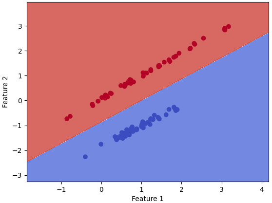
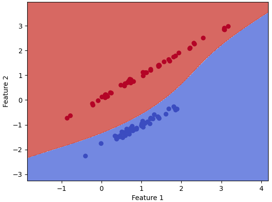
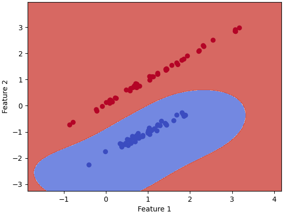
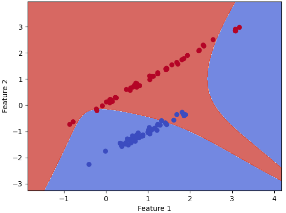
If we want to use different models as the training model for the ML analysis, we can just simply change the code line of "model = Perceptron()" to, for instance, "model = SVC() ", "model = GaussianNB()", and "model = KNeighborsClassifier(n_neighbors=2)" and "model = KNeighborsClassifier(n_neighbors=3)" for different neighbors (here are 2 neighbors and 3 neighbors.
Table 4312b. Applications which is not provided by Scikit-learn/sklearn.
| Application |
Details |
| Bessel Function kernel |
Scikit-learn does not provide a built-in Bessel Function kernel |
| Bayesian optimization |
Bayesian optimization can be applied in hyperparameter tuning, using the scikit-optimize library |
| Ensemble of decision trees |
Ensemble of decision trees can be done by using the scikit-learn library to implement decision trees and gradient boosting, which can be considered an additive model, with a decision tree for regression |
| Laplacian kernel |
Scikit-learn's SVM implementation doesn't provide a built-in Laplacian kernel option. |
Furthermore, "from sklearn.model_selection import train_test_split" is part of the scikit-learn library, which is a popular machine learning library in Python. The train_test_split function is commonly used to split a dataset into training and testing sets. This is a crucial step in machine learning model development to assess how well a model generalizes to new, unseen data:
from sklearn.model_selection import train_test_split
# Assuming X is our feature matrix and y is our target variable
X_train, X_test, y_train, y_test = train_test_split(X, y, test_size=0.2, random_state=42)
Here,
X is your feature matrix (input variables).
y is your target variable (output variable or labels).
test_size is the proportion of the dataset to include in the test split (e.g., 0.2 for 20%).
random_state is an optional parameter that allows you to set a seed for reproducibility.
The function returns four sets: X_train, X_test, y_train, and y_test, which are the training and testing sets for both features and target variables, respectively. The training set is used to train the machine learning model, and the testing set is used to evaluate its performance on new, unseen data.
Scikit-Learn is particularly popular for traditional machine learning and comes with a simple, consistent API that is ideal for newcomers and for deploying models quickly. Key API features include:
-
Estimator API, which is used across all learning algorithms in Scikit-Learn, ensuring consistency and simplicity. It standardizes the functions for building models, fitting them to data, and making predictions.
-
Transformers and Preprocessors for data scaling, normalization, and transformation, which are crucial for preparing data for training.
-
Pipeline API which helps in chaining preprocessors and estimators into a single coherent workflow, simplifying the process of coding and reducing the chance of errors.
-
Model Evaluation Tools which provide metrics, cross-validation, and other utilities to evaluate and compare the performance of algorithms.
|