=================================================================================
The discrepancy between predicted labels and true labels is used to calculate various metrics that quantify the model's accuracy and ability to generalize to new, unseen data.
The accuracy of supervised machine learning models is evaluated using various performance metrics and parameters, depending on the specific problem and the nature of the data. Some common parameters used to evaluate the accuracy of supervised machine learning models include:
-
Accuracy: This is the most straightforward metric and is simply the ratio of correctly predicted instances to the total number of instances. While easy to understand, accuracy can be misleading, especially when dealing with imbalanced datasets where one class is much more prevalent than others.
-
Precision: Precision measures the proportion of true positive predictions (correctly predicted positive instances) out of all positive predictions (both true positives and false positives). It indicates the model's ability to avoid false positives. High precision is desirable when false positives are costly.
-
Recall (Sensitivity or True Positive Rate): Recall calculates the proportion of true positive predictions out of all actual positive instances. It indicates the model's ability to capture all positive instances and avoid false negatives. High recall is important when false negatives are costly.
-
F1-Score: The F1-score is the harmonic mean of precision and recall. It provides a balanced measure of a model's performance by considering both false positives and false negatives. It is especially useful when there's a class imbalance.
-
Specificity (True Negative Rate): Specificity measures the proportion of true negative predictions (correctly predicted negative instances) out of all actual negative instances. It is the opposite of recall and is important when the cost of false negatives is low.
-
Area Under the ROC Curve (AUC-ROC): The ROC curve plots the true positive rate (recall) against the false positive rate for different classification thresholds. AUC-ROC quantifies the overall performance of a model across various thresholds. It is useful for binary classification tasks and provides insights into how well the model distinguishes between classes.
-
Area Under the Precision-Recall Curve (AUC-PR): Similar to AUC-ROC, the AUC-PR curve plots precision against recall for different thresholds. It is particularly informative for imbalanced datasets, where positive instances are rare.
-
Confusion Matrix: A confusion matrix provides a comprehensive view of a model's performance by showing the counts of true positive, true negative, false positive, and false negative predictions.
-
Mean Absolute Error (MAE): Used for regression tasks, MAE measures the average absolute difference between predicted and actual values. It gives an idea of the magnitude of the model's errors.
-
Mean Squared Error (MSE): Another regression metric, MSE calculates the average of the squared differences between predicted and actual values. It amplifies larger errors and is sensitive to outliers.
-
Root Mean Squared Error (RMSE): RMSE is the square root of MSE and is more interpretable in the original scale of the target variable.
-
R-squared (Coefficient of Determination): This metric explains the proportion of the variance in the target variable that is predictable from the independent variables. It helps assess how well the model fits the data.
Unsupervised machine learning involves tasks where the goal is to discover patterns, relationships, or structures within data without the use of labeled outputs. The evaluation of unsupervised machine learning models can be more challenging than in supervised learning, as there are no explicit ground truth labels to compare against. Nevertheless, there are several parameters and techniques used to assess the quality and effectiveness of unsupervised learning algorithms. Some of these parameters include:
-
Internal Evaluation Metrics:
- Silhouette Score: Measures how similar an object is to its own cluster (cohesion) compared to other clusters (separation).
- Davies-Bouldin Index: Measures the average similarity between each cluster and its most similar cluster, considering both intra-cluster and inter-cluster distances.
- Calinski-Harabasz Index (Variance Ratio Criterion): Compares the between-cluster variance to the within-cluster variance.
- Inertia or Within-Cluster Sum of Squares: Measures the sum of squared distances between data points and their cluster's centroid.
- External Evaluation Metrics:
- Adjusted Rand Index (ARI): Measures the similarity between the true labels and the predicted labels, correcting for chance.
- Normalized Mutual Information (NMI): Measures the mutual information between true and predicted labels, normalized to account for differences in cluster size.
- Fowlkes-Mallows Index: Measures the geometric mean of precision and recall between true and predicted clusters.
- Visualization Techniques:
- Principal Component Analysis (PCA): Projects high-dimensional data into a lower-dimensional space to visualize clusters.
- t-Distributed Stochastic Neighbor Embedding (t-SNE): Non-linear dimensionality reduction technique often used for visualizing clusters in lower-dimensional space.
- Hierarchical Clustering Dendrograms: Visual representation of the hierarchical structure of clusters.
- Comparative Analysis:
- Elbow Method: Used in K-means clustering, it identifies the optimal number of clusters by plotting the within-cluster sum of squares against the number of clusters and looking for the "elbow" point.
- Gap Statistic: Compares the performance of a clustering algorithm to a random distribution, helping to determine the appropriate number of clusters.
- Dendrogram Cutting: In hierarchical clustering, dendrograms can be cut at different levels to form clusters, and the results can be compared against known ground truth or other metrics.
- Domain Knowledge and Interpretability:
- Unsupervised learning results are often evaluated by experts in the domain to determine if the discovered patterns or structures make sense and provide valuable insights.
It's important to note that unsupervised learning is often more exploratory and subjective in nature compared to supervised learning, and the choice of evaluation parameters may vary depending on the specific goals of the analysis and the characteristics of the data. Additionally, there's no one-size-fits-all metric, and a combination of multiple evaluation techniques is often used to gain a comprehensive understanding of the model's performance.
Non-linearity helps in training your model at a much faster rate and with more accuracy without the loss of your important information.
Table 4085 shows the accuracy rates of the
tested algorithms in fault classification using machine learning.
| Table 4085. Accuracy rates of the
tested algorithms in fault classification using machine learning. |
| Classifier |
Accuracy |
Reference |
| Fine tree |
82.20% |
[1] |
| Medium tree |
79.40% |
[1] |
| Coarse tree |
55.20% |
[1] |
| Linear SVM |
52.50% |
[1] |
| Quadratic SVM |
78.20% |
[1] |
| Cubic SVM |
87.10% |
[1] |
| Fine Gaussian SVM |
63.60% |
[1] |
| Medium Gaussian SVM |
67.20% |
[1] |
| Coarse Gaussian SVM |
51.80% |
[1] |
============================================
The range of values that constitute "good" machine learning performance varies widely depending on the specific task, dataset, and domain. There is no universal threshold or fixed range for metrics like accuracy, precision, recall, or mean squared error (MSE) that applies to all machine learning projects. What's considered good performance depends on several factors:
-
Task Complexity: Simple tasks may require high accuracy, precision, recall, or low MSE, while more complex tasks might have more forgiving performance requirements.
-
Data Quality: High-quality, well-preprocessed data often leads to better model performance. In contrast, noisy or incomplete data may result in lower performance.
-
Imbalanced Data: In classification tasks with imbalanced class distributions, achieving a high accuracy might be misleading. In such cases, precision, recall, or F1-score for the minority class may be more important.
-
Domain Requirements: Different domains and applications have varying tolerances for errors. For example, in medical diagnosis, high recall (to minimize false negatives) is often crucial, even if it means lower precision.
-
Business Impact: Consider the real-world impact of model predictions. The consequences of false positives and false negatives can greatly influence what is considered acceptable performance.
-
Benchmark Models: Comparing your model's performance to a baseline or existing models in the field can help determine if your model is achieving a meaningful improvement.
-
Human-Level Performance: Sometimes, you may aim to achieve performance that is close to or even surpasses human-level performance on a task.
-
Application-Specific Metrics: Certain applications might have specific metrics tailored to their requirements. For example, in natural language processing, you might use metrics like BLEU or ROUGE for text generation tasks.
To determine what range of values constitutes good performance for your specific project, you should:
-
Set Clear Objectives: Clearly define what you aim to achieve with your model and how its predictions will be used in the real world.
-
Consult with Stakeholders: Discuss performance expectations and requirements with domain experts and stakeholders to ensure alignment with project goals.
-
Use Validation Data: Split your data into training, validation, and test sets. Use the validation set to tune hyperparameters and assess model performance.
-
Consider Trade-offs: Understand that there are often trade-offs between different performance metrics. Improving one metric may negatively impact another, so choose metrics that align with your project's priorities.
-
Iterate and Improve: Continuously monitor and improve your model's performance, considering feedback from stakeholders and real-world performance.
We can evaluate how well a prediction ŷ matches a given response y by utilizing a loss function denoted as Loss(y, ŷ). In regression scenarios, the common preference is the squared-error loss, expressed as (y - ŷ)^2. In the context of classification, the zero-one loss function, denoted as Loss(y, ŷ) = 1{y ≠ ŷ}, is frequently employed. This function assigns a loss of 1 whenever the predicted class ŷ doesn't match the true class y.
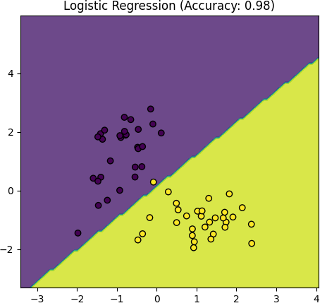
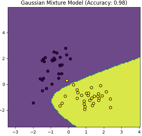
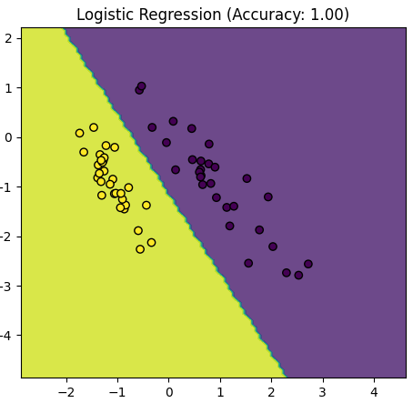
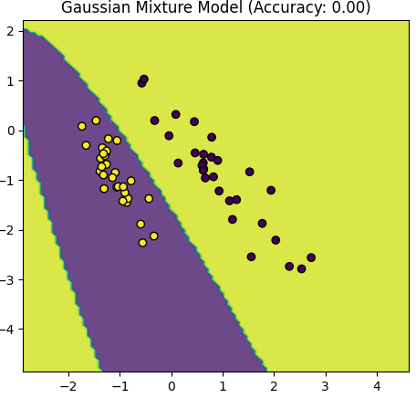
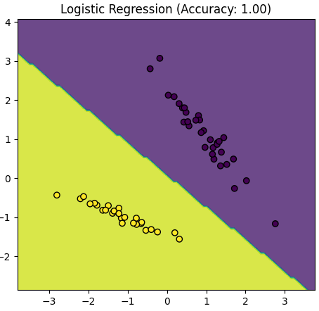
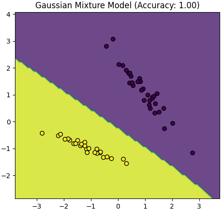
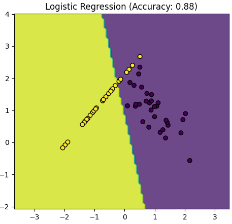
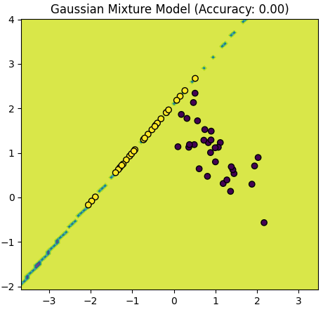
Table 4085. Comparison between Logistic Regression and Gaussian Mixture Model.
Logistic Regression |
Gaussian Mixture Model |
|
|
|
|
|
|
|
|
|
The script above provided in the earlier response is primarily focused on visualizing the data and the decision boundaries created by a Logistic Regression model and a Gaussian Mixture Model (GMM) for two distinct classes (positive and negative examples). It doesn't explicitly calculate and compare accuracy values for the models.
However, Logistic Regression might have a more stable accuracy compared to a GMM:
-
Simplicity of Logistic Regression: Logistic Regression is a discriminative model that is well-suited for binary classification tasks. It estimates a decision boundary that separates the classes, making it less sensitive to the underlying distribution of data. It often works well when the data is linearly separable.
-
Parameter Estimation: Logistic Regression has a well-defined algorithm for estimating model parameters (coefficients) that optimize a likelihood function. It's typically less sensitive to initialization and can converge to stable solutions.
-
Assumptions: GMM is a generative model that makes assumptions about the distribution of data. If these assumptions are not met or if the data is not well-suited for a Gaussian distribution, GMM might have difficulty modeling the data accurately. Additionally, GMM may require more careful initialization of parameters, and the number of components (clusters) must be specified in advance.
-
Complexity: GMM is a more complex model than Logistic Regression. It models data as a mixture of Gaussian distributions, which can be sensitive to the choice of covariance structure and initialization. Ensuring convergence and finding the correct number of components can be challenging.
To make a direct comparison of stability and accuracy between these two models, you would need to perform a more structured experiment, including cross-validation, multiple runs with different data splits, and potentially hyperparameter tuning. You would also need to calculate accuracy, precision, recall, and other relevant metrics to evaluate model performance.
In practice, the choice between Logistic Regression and GMM depends on the specific characteristics of the data and the problem you are trying to solve. Logistic Regression is typically preferred for standard classification tasks, while GMM is used when the data is better represented as a mixture of Gaussian distributions. The stability and performance of each model can vary based on the data and problem context.
|
============================================
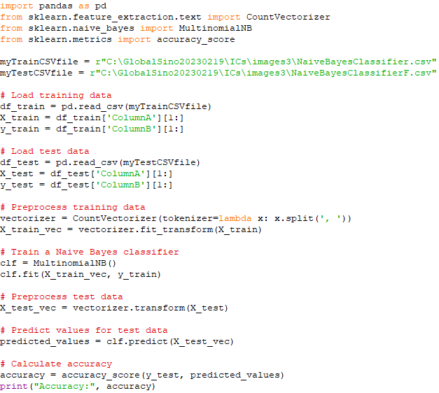
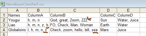
Test the accuracy of Machine learning with Naive Bayes algorithm with the current train model. To calculate accuracy, you need a test dataset with known labels (ground truth) that the model hasn't seen during training. Assuming you have a separate CSV file containing test data similar to your training data, here's how you can modify your code to calculate and print the accuracy of your Naive Bayes classifier. In this case below, I've preprocessed the test data using the same vectorizer that was fitted on the training data. After predicting values for the test data, the accuracy is calculated using the accuracy_score function from sklearn.metrics. This accuracy score represents the percentage of correct predictions on the test dataset. Code:
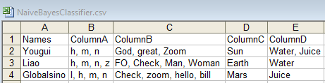
Group A:
Input A: Train:
Input B: Test (which is the same as the Train file):
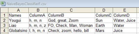
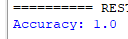
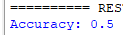
Output:
Group B:
Input A: Train:
Input B: Test (which is not the same as the Train file):
Output (due to the differences between Test and Train files, the accuracy is lower now):
[1] Balamurali Krishna Ponukumati, Pampa Sinha, Manoj Kumar Maharana, A. V. Pavan Kumar and Akkenaguntla Karthik, An Intelligent Fault Detection and Classification Scheme for Distribution Lines Using Machine Learning, Engineering, Technology & Applied Science Research, 12(4), pp.8972-8977, (2022).
|