=================================================================================

In machine learning and probability theory, a joint probability distribution refers to the probability distribution that describes the simultaneous occurrence of multiple random variables. It quantifies the likelihood of specific outcomes or combinations of outcomes for all the random variables considered together.

Let's break down the notation "p over the space of x times y":

1. "p" represents the probability or likelihood.

2. "x" and "y" are random variables. These variables can represent different events, features, or measurements in a probabilistic model. "x" and "y" can take on various values, and the joint probability distribution describes how likely different combinations of values for "x" and "y" are.

3. "times" here simply denotes that we are considering the joint probability distribution of "x" and "y" together, not separately. It implies that we are interested in understanding the probability of specific outcomes for both "x" and "y" occurring together.

4. "space of x times y" refers to the combined set of all possible values or outcomes that "x" and "y" can jointly take. This space represents all possible pairs or combinations of values that "x" and "y" can have.

For example, if you have two random variables, "x" representing the temperature and "y" representing humidity, the joint probability distribution "p(x, y)" would describe how likely it is for specific temperature-humidity pairs to occur together. It specifies the probability of observing a particular temperature and humidity value simultaneously.

The joint probability distribution is fundamental in various machine learning tasks, including probabilistic modeling, Bayesian inference, and graphical models like Bayesian networks. It provides a way to model and reason about the relationships between multiple random variables in a probabilistic manner.

A joint probability distribution can be explained using a table known as a probability distribution table. This table shows the probabilities associated with different combinations of values for multiple random variables. Let's use a simple example to illustrate this concept.

Suppose we have two discrete random variables, "X" and "Y," each with three possible outcomes. We want to calculate and represent their joint probability distribution.

Here's a probability distribution table for "X" and "Y":

          | X | Y | P(X, Y) |
          |-------|-------|----------|
          | x1 | y1 | P(X=x1, Y=y1) |
          | x1 | y2 | P(X=x1, Y=y2) |
          | x1 | y3 | P(X=x1, Y=y3) |
          | x2 | y1 | P(X=x2, Y=y1) |
          | x2 | y2 | P(X=x2, Y=y2) |
          | x2 | y3 | P(X=x2, Y=y3) |
          | x3 | y1 | P(X=x3, Y=y1) |
          | x3 | y2 | P(X=x3, Y=y2) |
          | x3 | y3 | P(X=x3, Y=y3) |

In this table:

• "X" and "Y" are the random variables, and they have three possible values each (x1, x2, x3 for X and y1, y2, y3 for Y).

• "P(X, Y)" represents the joint probability of observing a specific combination of values for "X" and "Y." Each cell in the table contains the probability value associated with the corresponding pair of values for "X" and "Y."

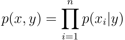
For instance, if we wanted to find the joint probability of "X" taking the value x2 and "Y" taking the value y3, we would look at the cell in the table corresponding to row "x2" and column "y3," which would give us P(X=x2, Y=y3).

This table allows you to quantify and visualize the joint probabilities of all possible combinations of values for the random variables "X" and "Y," providing a comprehensive representation of their joint probability distribution.

The joint probability distribution of n random variables x₁, x₂, ..., x_n, conditioned on the variable y can be given by,

          -------------------------------- [3989a]

The equation states that the joint probability distribution of all the x variables, denoted as p(x, y), can be expressed as the product of the conditional probability distributions of each x variable given y, i.e., p(x_i|y), where i ranges from 1 to n.

Product rule in probability theory gives,

          -------------------------------- [3989b]

where,

1. p(x, y) is the joint probability, which represents the probability that both events x and y occur simultaneously.
2. p(x|y) is the conditional probability of event x occurring given that event y has already occurred. It quantifies the probability of x happening under the condition that y is known to have occurred.
3. p(y) is the marginal probability of event y, which is the probability of y occurring on its own, without any reference to event (x).

This equation expresses how the joint probability p(x, y) of two events or random variables x and y can be calculated in terms of the conditional probability p(x|y) of x given y and the marginal probability p(y) of (y).

============================================