Cross Entropy (Log Loss/Logistic Loss) - Python for Integrated Circuits - - An Online Book - |
||||||||
| Python for Integrated Circuits http://www.globalsino.com/ICs/ | ||||||||
| Chapter/Index: Introduction | A | B | C | D | E | F | G | H | I | J | K | L | M | N | O | P | Q | R | S | T | U | V | W | X | Y | Z | Appendix | ||||||||
================================================================================= Cross entropy is a concept often used in information theory and statistics, particularly in machine learning and data science. Cross entropy, also known as log loss or logistic loss, is a common mathematical concept used in machine learning and information theory to measure the dissimilarity between two probability distributions. In machine learning, it is often used as a loss function to evaluate the performance of classification models, particularly in binary and multi-class classification problems. Cross entropy is a way to measure the dissimilarity or the difference between two probability distributions. In machine learning, it's commonly used when comparing the predicted probability distribution generated by a model to the true probability distribution of the data:
Where: The result is a non-negative value, and it quantifies how well the estimated distribution Q represents the true distribution P. Lower cross-entropy indicates a better match between the two distributions. The loss function cross entropy can be used for classification problems. Here's how cross entropy works:
Here, "y" represents the class label (0 or 1), and the sum is taken over both classes. This formula penalizes the model more when it makes incorrect predictions with high confidence.
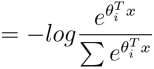
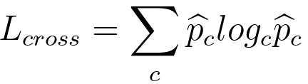
Here, the sum is taken over all C classes. The goal in machine learning is to minimize the cross-entropy loss. When your model's predicted probabilities match the true probabilities (i.e., when Q(y) equals P(y)), the cross-entropy loss is minimized to zero. However, as the predicted probabilities diverge from the true probabilities, the loss increases, indicating that the model's predictions are becoming less accurate. In practice, optimizing cross entropy is a common approach for training classification models using techniques like logistic regression, neural networks, and softmax regression. It encourages the model to produce accurate and well-calibrated probability estimates for each class, making it a popular choice as a loss function for classification tasks. For decision trees, with the theory of cross entropy loss, we have, :where,
The formula is essentially calculating the average negative log-likelihood of the true class labels given the predicted probabilities. It is commonly used as a loss function in classification problems, including those involving decision trees. Assuming there are two children regions R1 and R2, Figure 3979a shows the plot of cross entropy loss in Equation 3979e
In the scenario of splitting a dataset into two subsets (R1 and R2) based on a certain feature, assuming a dataset (Rp = 700 positive, Rn = 100 negative), which means there are 700 positive cases and 100 negative cases in the dataset, then we consider two possible splits: R1 = 600 positive, and R2 = 100 negative. R1 = 400 positive and 100 negative, and R2 = 200 positive. The logarithm in the cross-entropy loss function does not need to be base 2. The base of the logarithm depends on the context and the choice made during the formulation of the loss function. In most machine learning frameworks and applications, the natural logarithm (base e) is commonly used. The cross-entropy loss for a binary classification problem is often defined as: where, is the true label (either 0 or 1). is the predicted probability of the positive class. The logarithm in this formula is commonly the natural logarithm. For multi-class classification problems, the cross-entropy loss is extended to handle multiple classes. The formula becomes: where, is the true probability distribution (i.e., a one-hot encoded vector representing the true class). is the predicted probability distribution. The use of cross-entropy as an error metric, especially in machine learning and classification tasks, is a common and widely accepted practice. Cross-entropy is related to Shannon's information theory and is particularly suited for evaluating the performance of models that output probabilities. The binary cross-entropy formula, commonly used for binary classification problems is given by,
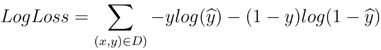
where,
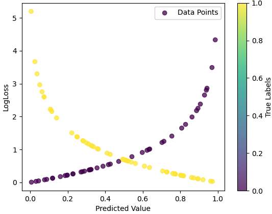
The formula sums over all data points in the dataset D, and for each data point, it calculates the cross-entropy loss between the true label y and the predicted probability y^. The loss penalizes the model more when its prediction is far from the true label. The term on the right-hand side in Equation 3979h is essentially a combination of two log loss terms, one for each class (0 and 1). The log loss penalizes confidently wrong predictions more than uncertain or correct predictions. This script at code plots predicted values versus LogLoss as shown in Figure 3979b. This script generates random true labels and predicted values for a binary classification problem and calculates the log loss for each data point.
Figure 3979b. Predicted values versus LogLos. The log loss is calculated for each data point using the formula in Equation 3979h. The formula penalizes predictions that are far from the true label, and it is commonly used as an evaluation metric for classification models. That is, the formula for log loss penalizes predictions based on the discrepancy between the predicted probability and the true label, for instance:
This behavior reflects the desire for the model to make confident and accurate predictions. Predictions that are closer to the true label result in lower log loss values, while predictions that are further away result in higher log loss values. For simplification, we can ignore the sum sign in Equation 3979h. Consider a scenario with one data point from a binary classification problem:
Substituting the given values into the equation, then we have,
Therefore, for this specific data point, with a true label of 1 and a predicted probability of 0.8, the log loss is approximately 0.2231. In the plotted figure, the x-coordinate will be 0.8 (predicted probability) and the y-coordinate will be 0.2231 (log loss). This point on the graph represents the relationship between the predicted value and the log loss for this particular data point. ============================================
|
||||||||
| ================================================================================= | ||||||||
|
|
||||||||
 ----------------------------------------------------- [3979b]
 --------------------------------- [3979e]
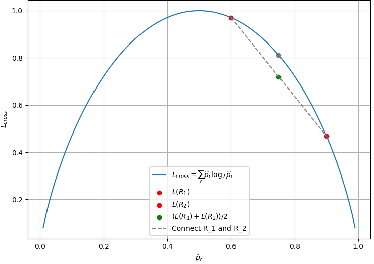
 ------------------------------- [3979h]