Non-asymptotic Analysis - Python for Integrated Circuits - - An Online Book - |
||||||||
| Python for Integrated Circuits http://www.globalsino.com/ICs/ | ||||||||
| Chapter/Index: Introduction | A | B | C | D | E | F | G | H | I | J | K | L | M | N | O | P | Q | R | S | T | U | V | W | X | Y | Z | Appendix | ||||||||
================================================================================= Non-asymptotic analysis is a mathematical and statistical approach that focuses on analyzing the behavior of algorithms, models, or systems for finite or specific input values, as opposed to asymptotic analysis, which studies their behavior as input values tend toward infinity. In non-asymptotic analysis, you aim to provide precise, often worst-case, bounds or estimates of performance, error rates, or other relevant quantities within a fixed range of input values. This approach is particularly important when dealing with practical and real-world applications where input values are limited and finite. Here are some key points about non-asymptotic analysis:
In summary, non-asymptotic analysis is a valuable approach for understanding the behavior of algorithms, models, or systems in real-world situations with finite input values. It provides precise and practical insights that are crucial for making informed decisions in various fields, including computer science, engineering, statistics, and machine learning. In non-asymptotic analysis, particularly in the context of theoretical computer science and machine learning, O(x) refers to a notation that quantifies the behavior of an algorithm, data structure, or computational process in terms of its resource usage or performance with respect to a specific input size x. This notation is used to describe the upper bound on the resource consumption or runtime of an algorithm as a function of the input size, without making any asymptotic assumptions like those made in big O notation (e.g., O(n), O(log n), O(1)). Here's how O(x) is typically used in non-asymptotic analysis:
For example, if you have a sorting algorithm and you want to know its worst-case runtime for sorting exactly 100 elements, you might express this as O(100), indicating that the algorithm's worst-case runtime is bounded by some constant when sorting 100 elements. When you write O(x), you're indicating the upper bound of a function (f(x)) in terms of its absolute value for all real values of x, and this upper bound is constrained by a constant factor (C) that may depend on x. Here's a mathematical representation of the statement: For every function f(x), we can write: O(x) = { g(x) : |f(x)| ≤ Cx, for all x ∈ ℝ } ------------------------------------------------- [3961a] In this equation:
Equation 3961 tells, when you write O(x), you're essentially saying that there exists a constant Cx such that the absolute value of the function f(x) is bounded by Cx times x for all real values of x. This notation is commonly used in non-asymptotic analysis to describe the behavior of functions with respect to their inputs. L(θ^) - L(θ) ≤ O(f(p, n)) ------------------------------------------------ [3961b] Equation 3961b represents a relationship between the difference in likelihoods and a bound based on a function of parameters p and n. L^(θ) ≈ L(θ) in some sense ------------------------------------------- [3961c] Equation 3961c in machine learning is referring to the relationship between an estimator's risk and its true risk, often in the context of non-asymptotic analysis:
Case 1: Suppose |L^(θ) - L(θ*)| ≤ α, and L(θ^) - L^(θ^) ≤ α; then L(θ^) - L(θ*) ≤ 2α. That means you can bound the excess rates by 2 times α. Explanation: In this context, we have two loss functions, L^(θ) and L(θ*), and two parameter values, θ and θ^, respectively. The statement sets up two conditions:
The conclusion is as follows: Proof: Let's start with the conditions:
We want to prove that:
Now, let's add condition 1 and condition 2 together: (L^(θ) - L(θ*)) + (L(θ^) - L^(θ^)) ≤ α + α ------------------------------------------ [3961g] Now, rearrange the terms: L(θ^) - L(θ*) + (L^(θ) - L^(θ^)) ≤ 2α ------------------------------------------ [3961h] Now, notice that we have L^(θ) - L^(θ^) on the left side. This is a common term in both conditions 1 and 2. We can replace it with α using condition 2: L(θ^) - L(θ*) + α ≤ 2α ------------------------------------------ [3961i] Now, subtract α from both sides: L(θ^) - L(θ*) ≤ 2α - α ------------------------------------------ [3961j] Simplify: L(θ^) - L(θ*) ≤ α ------------------------------------------ [3961k] So, we have proven that: L(θ^) - L(θ*) ≤ α ------------------------------------------ [3961l] This shows that you can indeed bound the excess rates of the loss functions L^(θ) and L(θ*) by 2α, as stated in the original statement. Therefore, the statement is proven by starting with the given conditions and manipulating them to show that the excess rate of L(θ^) - L(θ*) is strictly less than or equal to 2α when both conditions are satisfied, which is the desired result. This result is important in non-asymptotic analysis in machine learning as it provides a bound on how much two loss functions can differ given certain conditions on their differences from a reference value. In nonasymptotic analysis, when you define σ^2 (sigma squared) as: This equation represents the variance of a sample of n data points, where a_i and b_i are the ith elements of two datasets, and σ^2 represents the squared difference between these datasets normalized by n. The standard deviation σ can be viewed as an upper bound on the typical or maximum deviation between the values of the random variables bi and ai in the sample. Here's why:
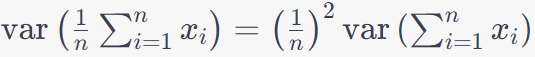
In summary, σ can be viewed as an upper bound on the typical deviation between the values bi and ai in your sample. It provides a measure of how much individual values typically deviate from the mean, and this can be useful for understanding the variability and potential extreme values in your dataset, particularly when applying probabilistic bounds like Chebyshev's inequality. You can use the properties of variance. The variance of a constant multiplied by a random variable is equal to the constant squared times the variance of the random variable. In this case, the constant is 1/. This equation tells us: Sample Size (): The term 1/ in the equation indicates that as the sample size () increases, the variance of the sample mean decreases. In other words, larger sample sizes provide a more precise estimate of the population mean because the individual data points have less influence on the sample mean's variability. Individual Variances ): The term represents the variance of each individual data point xi. The summation Independence and Identical Distribution (i.i.d.): The equation assumes that the values are independent and identically distributed (i.i.d.). In other words, each is a random variable from the same probability distribution with the same variance. Population Variance: The equation gives insight into how the variance of the sample mean relates to the variance of the individual data points. It's a key formula in statistics because it connects the precision of sample estimates to the variability of the underlying population. In practical terms, this formula is used to assess the precision of sample means in statistics. It tells you how much the sample mean is expected to vary from one sample to another, given the sample size and the individual data point variances. A smaller variance of the sample mean indicates that the sample mean is a more reliable estimate of the population mean. Now, we have the equation below: where,
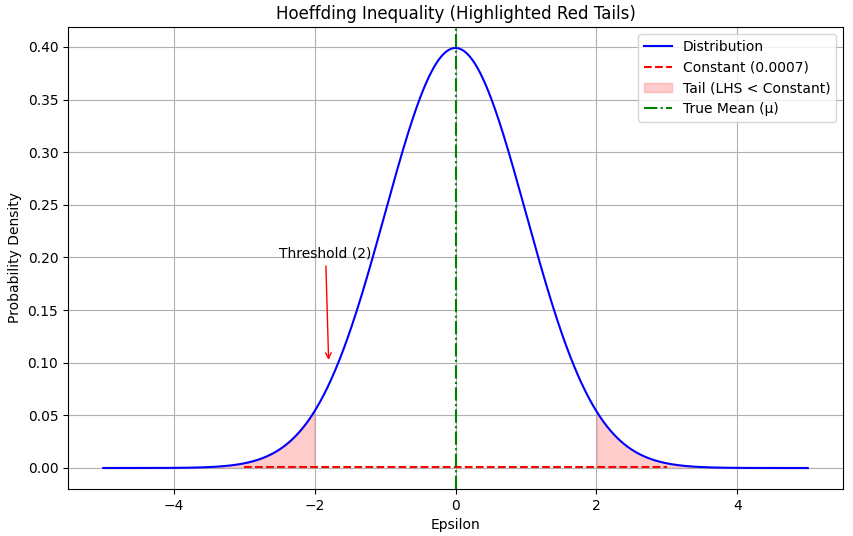
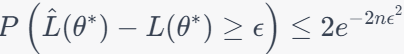
Now, we use a constant related to , , and to define : This is a threshold which is a value that represents a significant deviation from the expected mean (μ). where, is slightly larger than the standard deviation () scaled by the square root of the logarithm of . The Hoeffding inequality is then applied with as a large constant: Here, represents probability, is the expected value, and is the value we defined in the previous equation. In the most interesting regime, when is plugged in: The left side represents the probability that the sample mean exceeds a certain threshold, which is given by . The range of this probability depends on the characteristics of your data and the specific values of , , and . The right side of the inequality is a constant term. This constant has a fixed value and is not affected by changes in your data. It's approximately equal to 0.13534 when c2/σ2 = 1. The range of the inequality is such that the probability on the left side is greater than or equal to the constant on the right side. In other words, it sets an upper bound on how likely it is for the sample mean to exceed the threshold determined by . We have: This shows how is defined and how it is used in the Hoeffding inequality, providing bounds on the probability of deviations from the mean. Keep in mind that this is an approximation and will converge better when −2c2/σ2 is large, implying a very low probability of an extreme deviation. Inequality 3961q describes a probabilistic relationship between the sample mean (), the true mean (), and a threshold (). It suggests that the probability of observing a sample mean less than or equal to � is greater than or equal to the constant 2e-2c^2/σ^2. Probability Distribution: Imagine the probability distribution of your sample mean. It might be a bell-shaped curve (if the sample size is sufficiently large due to the Central Limit Theorem) or some other distribution depending on your data and assumptions. True Mean (): This represents the expected value of your sample mean under ideal conditions, i.e., the mean of the distribution. Threshold (): This is a threshold value that you set based on your analysis. It represents a specific level below which you want to make inferences. Hoeffding Inequality Visualization. Code: You can apply the Hoeffding inequality to the difference between the empirical (sample) loss and the true (population) loss, often represented as Where:
If , where represents an estimated or sample parameter and * represents the true or population parameter, the difference between the estimated loss () and the true loss () will be zero. In mathematical terms, this can be expressed as: In this case, the estimated parameter () is equal to the true parameter (), which means that your estimation is perfectly accurate. As a result, the difference between the empirical (sample) loss () and the true (population) loss () is zero because there is no discrepancy between the estimated and true parameter values. In practical terms, this scenario represents an ideal case where your estimation method provides an exact match to the true parameter value, and there is no bias or error in your estimation. However, in many real-world situations, it is challenging to achieve such perfect accuracy, and estimators are subject to various sources of error and uncertainty. The Hoeffding inequality and related statistical techniques are often used to quantify and control the uncertainty associated with parameter estimation. The estimator depends on the sample data. In statistics and parameter estimation, is a function of the observed sample values and is used to estimate an unknown parameter based on the available data. The estimator is computed from the sample data and represents your best guess or estimate of the true parameter . The specific form of depends on the estimation method used, which can vary depending on the statistical problem and the nature of the data. ============================================
|
||||||||
| ================================================================================= | ||||||||
|
|
||||||||
 ----------------------------- [3961n]
 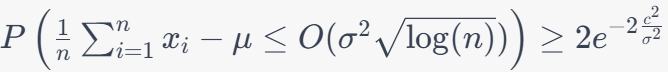 ----------------------------- [3961p]
 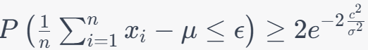 -------------- [3961q]
 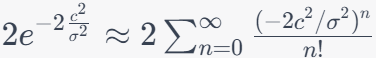 ------------- [3961r]
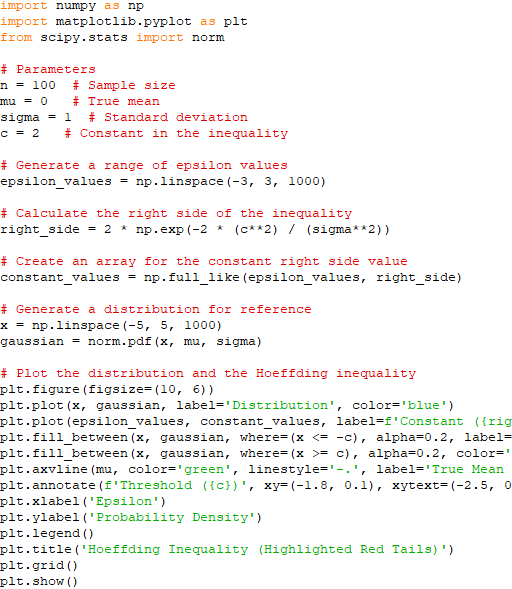
 ------------- [3961s]