=================================================================================

In probability theory, complementary inequalities are a way to express the relationship between the probability of an event occurring and the probability of its complementary event (the event not occurring):

1. Original Inequality: For an individual hypothesis ℎ from the hypothesis class H, the original inequality asserts:

   P(Event) ≥ 1 − δ ------------------------------------------------ [3941a]

   Here, "P(Event)" represents the probability that the event of interest occurs for a particular hypothesis ℎ, and "δ" is a small positive value (usually a small probability) that represents the allowed probability of error or failure.

   This inequality essentially states that the probability of the event happening should be greater than or equal to 1 minus the allowed error probability δ. In other words, you want the event to occur with high probability, which is 1 - δ.

2. Complementary Inequality: The complementary inequality asserts that the opposite event occurs with high probability:

   P(Opposite Event) ≤ δ ----------------------------------------------- [3941b]

   Here, "P(Opposite Event)" represents the probability that the opposite (complementary) event, which is the event not occurring, happens for the same hypothesis ℎ. Again, "δ" is the allowed error probability.

   This inequality focuses on quantifying the probability of the opposite event (not occurring) being less than or equal to δ. In other words, it ensures that the event doesn't happen with a probability greater than δ.

These two inequalities work together to ensure that the event of interest and its complementary event are controlled with respect to the allowed error probability δ. If you can guarantee that the event occurs with high probability (Original Inequality), you can simultaneously quantify that the opposite event (not occurring) happens with low probability (Complementary Inequality), given the same hypothesis ℎ.

This approach is fundamental in various fields, including statistics, machine learning, and hypothesis testing, where you want to manage the trade-off between ensuring an event's occurrence and quantifying the risk of it not happening.

The concepts of complementary inequalities are indeed used in machine learning, particularly in the context of statistical learning theory and hypothesis testing. Here are some examples of how these concepts are applied in machine learning:

1. Confidence Intervals: In machine learning, confidence intervals are often used to quantify uncertainty around model predictions or parameter estimates. The original inequality corresponds to the confidence interval's lower bound (for the event of interest), and the complementary inequality corresponds to the upper bound (for the complementary event). This allows practitioners to express the confidence that a model's prediction falls within a certain range.

2. Hypothesis Testing: In hypothesis testing, you may want to test whether a particular hypothesis is true or not based on data. The original inequality can be used to specify the null hypothesis (the event of interest) and the complementary inequality specifies the alternative hypothesis (the opposite event). Statisticians use these inequalities to calculate p-values and make decisions about hypothesis acceptance or rejection.

3. Error Bounds in Machine Learning Models: When training machine learning models, you often want to control the error rate. The original inequality can represent the desired accuracy (event of interest), and the complementary inequality can be used to control the error rate (false positives or false negatives) within a specified limit.

4. Statistical Learning Theory: In the context of statistical learning theory, the original inequality relates to the concept of "probably approximately correct" (PAC) learning. It states that a learning algorithm should find a hypothesis that is probably accurate with high probability. The complementary inequality quantifies the probability of failure in this context.

5. Boosting Algorithms: Algorithms like AdaBoost and gradient boosting often use weighted versions of the complementary inequality to focus on examples that were misclassified in previous rounds of training. By emphasizing the examples that are harder to classify, these algorithms can improve overall model performance.

6. Reinforcement Learning: In reinforcement learning, where agents learn from interactions with an environment, these concepts can be used to specify desired probabilities of taking certain actions or achieving specific outcomes, while also quantifying the risk of undesirable actions or outcomes.

These are just a few examples of how complementary inequalities are employed in machine learning to manage uncertainty, control errors, and make probabilistic assertions about events and outcomes. They play a crucial role in model evaluation, statistical analysis, and decision-making within the field of machine learning.

============================================

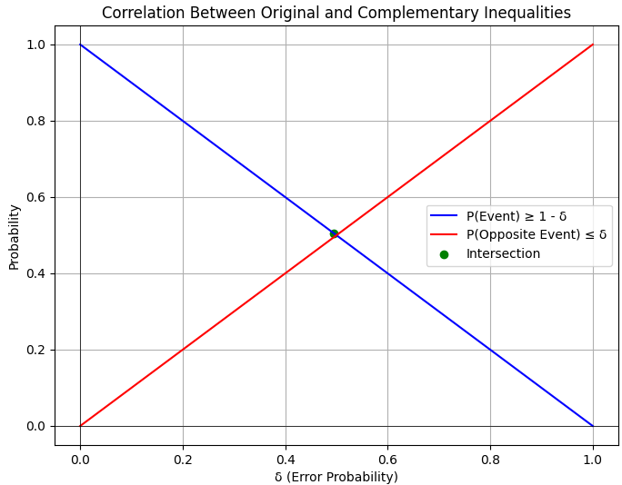
Complementary Inequality. Code:
         
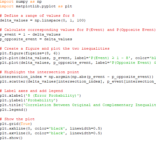
       Output: