=================================================================================
Locally Weighted Regression (LWR), often referred to as Locally Weighted Scatterplot Smoothing (LOWESS) or LOcally Weighted Polynomial Regression (LOESS), is a non-parametric and adaptive regression technique used in statistics and machine learning for modeling the relationship between a dependent variable (the target) and one or more independent variables (predictors or features). It is particularly useful when dealing with data that doesn't follow a simple linear or polynomial relationship and exhibits complex, non-linear patterns.
The key idea behind LWR is to give more weight to data points that are closer to the point where you want to make a prediction. In other words, LWR fits a separate regression model for each data point, and the contribution of each data point to the prediction is determined by its proximity to the point of interest. The closer a data point is to the point being predicted, the more influence it has on the model:
-
For each prediction point, LWR defines a local region around it by specifying a bandwidth or a window size. This region contains the training data points that are considered relevant for making a prediction at that point.
-
LWR assigns weights to the training data points within the local region. Typically, it uses a kernel function, such as the Gaussian kernel, to assign higher weights to data points closer to the prediction point and lower weights to those farther away. The kernel function ensures that data points closer to the prediction point have a stronger influence on the model.
-
A weighted regression model (usually linear regression) is then fitted within the local region. The model parameters are estimated based on the weighted data points.
-
To make a prediction at a new point, LWR repeats the process: it identifies the relevant local region around the new point, assigns weights to the training data points within that region, and fits a regression model using the weighted data.
Advantages of Locally Weighted Regression:
- LWR can capture complex, non-linear relationships in the data because it adapts to the local patterns.
- It doesn't assume a fixed functional form for the relationship, making it versatile for various types of data.
- LWR is suitable for non-linear relationships: LWR is a non-parametric regression technique that models the relationship between variables in a data set without assuming a specific functional form, such as a linear relationship. It works well when the relationship between the variables is non-linear.
- For low-dimensional data set: we tend to use LWR when we have a relatively low-dimensional data set
- Flexibility in modeling: LWR adapts to the local characteristics of the data. In a low-dimensional data set, it is often easier to capture the local relationships between variables because there are fewer dimensions to consider. LWR can adapt well to these local nuances.
- Overfitting is less of a concern: In high-dimensional data sets, traditional regression models like linear regression can easily overfit the data, leading to poor generalization to new data. LWR, on the other hand, tends to be less susceptible to overfitting, especially when applied to low-dimensional data. It focuses on the local region around each data point, which helps prevent overfitting.
- Reduced computational complexity: LWR can be computationally intensive, especially in high-dimensional spaces. In low-dimensional data sets, the computational burden is generally lower, making LWR a more practical choice.
- Data visualization and interpretation: In low-dimensional data, it's often easier to visualize and interpret the results of LWR. You can create scatterplots or other visualizations to see how the model behaves locally, which can be informative for understanding the data.
Disadvantages and Considerations:
- LWR can be computationally expensive, especially when making predictions for many points, as it requires fitting multiple regression models.
- The choice of the bandwidth parameter is critical, as it determines the size of the local region and affects the trade-off between bias and variance in the model.
- LWR is sensitive to outliers, as data points with large deviations from the prediction point can have a disproportionate impact on the model.
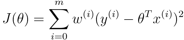
In Locally Weighted Regression (LWR), the goal is to fit the parameter vector θ in such a way that it minimizes the weighted sum of squared errors (also known as the cost function). The specific cost function that LWR aims to minimize is as follows:
 ------------------------------------------------------- [3891a] ------------------------------------------------------- [3891a]
where,
- J(θ) is the cost function that we want to minimize.
- Σᵢ represents the summation over all the data points i in your dataset.
- w(i) is a weight function assigned to the i-th data point. In LWR, the weights are typically determined by a kernel function that assigns higher weights to data points that are closer to the point at which you want to make a prediction.
- y(i) is the target or output value associated with the i-th data point.
- θT is the transpose of the parameter vector θ.
- x(i) is the feature vector associated with the i-th data point.
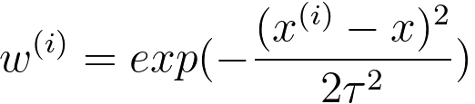
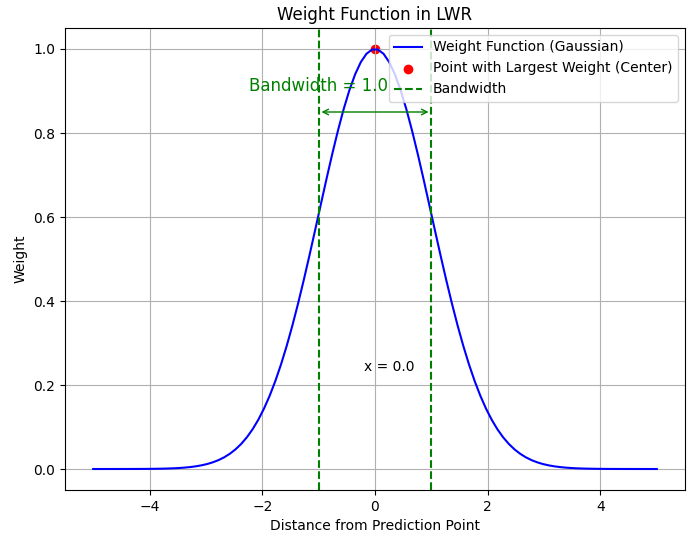
The common choice of w(i), shows in Figure 3891a, is,
 --------------------------------------------------- [3891b] --------------------------------------------------- [3891b]
where,
(a)
(b)
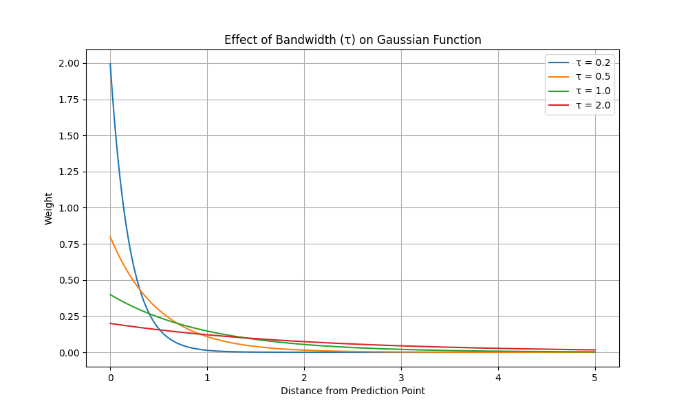
| Figure 3891b. (a) Weight Function (w(i)) in LWR (Python code), and (b) effect of bandwidth (τ) on gaussian function (Python code). The red dot stands for the feature vector associated with the i-th data point. The bandwidth (τ) is shown in the figure as well. |
If |x(i)-x| is small, then w(i) is close to 1, based on Equation 3891b. On the other hand, if |x(i)-x| is large,, then w(i) is close to 0. That means if x(i) is far away from x, then J(θ) becomes 0, based on Equation 3891a. In other words, the idea behind LWR is to give more weight to data points that are closer to the point where you want to make a prediction, effectively making the regression locally adaptive. This means that for each prediction, a different set of data points contributes more to the cost function, depending on their proximity to the point of interest.
The parameter vector θ is adjusted to minimize this weighted sum of squared errors, leading to a model that fits the data well in the local neighborhood of the prediction point while potentially ignoring data points that are far away. LWR is often used for non-parametric regression tasks when you want to capture complex and nonlinear relationships in the data, but the choice of the kernel and bandwidth parameters can significantly impact its performance.
Note that the bandwidth parameter (often denoted as τ or h) in locally weighted regression (LWR) and kernel density estimation (KDE) have an effect on the trade-off between overfitting and underfitting.
============================================
Locally Weighted Regression (LWR). Code:

Output:

============================================
|