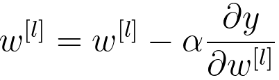
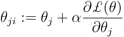
=================================================================================

In machine learning, when you want to update the parameters θ_j of a model using the gradient of the loss function ℒ(θ) with respect to θ_j, you typically use an optimization algorithm such as gradient descent. The update rule for θ_j is based on the gradient of the loss function and is designed to minimize the loss function over the training data.

The general update rule for θ_j using the gradient of the loss function is as follows:

          -------------------------------------------- [3875a]

Where:

• θ_j is the current (old) value of the parameter θ_j.
• θ_ji is the updated (new) value of the parameter θ_j.
• α is the learning rate, which is a hyperparameter that controls the step size of the update. It is typically a small positive value.
• ∂ℒ(θ) /∂θ_j is the partial derivative of the loss function ℒ(θ) with respect to θ_j. This represents the slope of the loss function with respect to the parameter θ_j.

The idea is to move the parameter θ_j in the direction that decreases the loss function. The size of the step is controlled by the learning rate α.

To update all the parameters of your model simultaneously, you would apply this update rule for each parameter θ_j in the model. This process is typically repeated for multiple iterations or until a convergence criterion is met (e.g., the change in the loss function becomes very small).

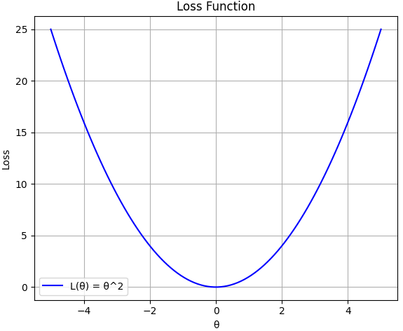
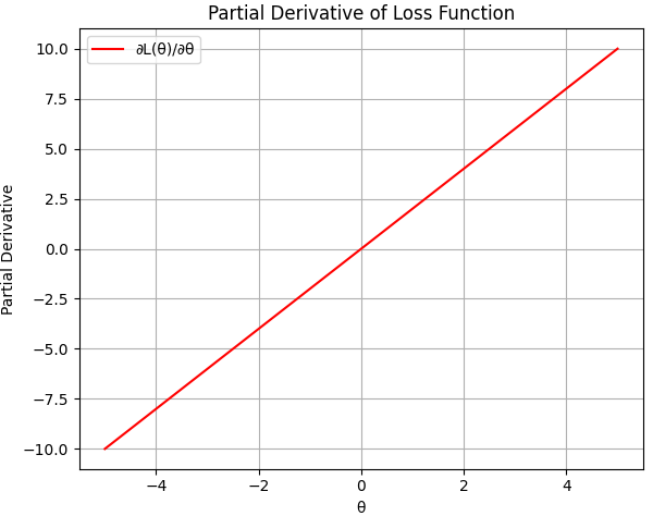
(a)

(b)

Figure 3875a. (a) Loss function, and (b) its partial derivative of θ² (Python script).

One example about the updated probability distribution of parameters or hypotheses is that in Bayesian statistics, the posterior distribution, which represents the updated probability distribution of parameters or hypotheses based on observed data, can be given by,

          P(θ|D) ∝ P(D|θ) * P(θ) ---------------------------------- [3875b]

where:

• P(θ|D) is the posterior distribution of the parameter θ given data D.
• P(D|θ) is the likelihood of observing data D given parameter θ.
• P(θ) is the prior distribution of the parameter θ.
• ∝ denotes proportionality, indicating that the right-hand side is proportional to the left-hand side.

For instance, in neural network, we update:

          ------------------------------------ [3875c]

Once the cost function is obtained, we can then plug in the cost function back in the gradient decent update rule and then update the weight parameter. For instance, in machine learning, particularly in the training of neural networks using gradient descent, the process typically involves the following steps:

1. Forward Pass: The input data is passed through the network, and the output is computed.

2. Compute Cost Function: The cost function, also known as the loss function, measures the difference between the predicted output and the actual target. It quantifies how well or poorly the model is performing.

3. Backward Pass (Backpropagation): The gradient of the cost function with respect to the model parameters (weights and biases) is computed. This involves applying the chain rule of calculus to propagate the error backward through the network.

4. Update Parameters: The parameters (weights and biases) of the model are updated using an optimization algorithm, typically gradient descent. The update rule is based on the gradients computed during the backward pass.

The gradient descent update rule is generally of the form:

          New parameter = Old parameter − Learning Rate × Gradient of the cost function with respect to the parameter ------ [3875d]

This process is repeated iteratively until the model converges to a state where the cost function is minimized.

In programming, assuming we have a defined gradient_descent function, to plot a graph with weights (w) or parameters (θ) versus cost function, we often need to store each w or θ in a list. On the other hand, for the ML modeling, we only need to return the last w value. To do this, this code is implementing a gradient descent algorithm and plots the cost function over the iterations, and stores each value of w/θ in a list. However, only the last value is stored with reinitialization or overwriting inside a loop so that only the final value is preserved to use in the ML process.

============================================