|
||||||||
Gaussian Discriminant Analysis (GDA) - Python and Machine Learning for Integrated Circuits - - An Online Book - |
||||||||
| Python and Machine Learning for Integrated Circuits http://www.globalsino.com/ICs/ | ||||||||
| Chapter/Index: Introduction | A | B | C | D | E | F | G | H | I | J | K | L | M | N | O | P | Q | R | S | T | U | V | W | X | Y | Z | Appendix | ||||||||
================================================================================= Gaussian Discriminant Analysis (GDA) is a classification algorithm used for supervised learning tasks and it can be used for prediction in the supervised machine learning tasks. It is closely related to Linear Discriminant Analysis (LDA) but assumes that the features follow a Gaussian distribution. In GDA, you model the probability distributions of the features for each class and then use these distributions to make predictions. Specifically, GDA estimates the parameters of the Gaussian distribution (mean and covariance) for each class and then uses these estimates to calculate the likelihood of a new data point belonging to each class. It's a generative model that can be used for both binary and multiclass classification problems. In GDA, we typically have a dataset with labeled examples. Each example is represented by a feature vector and an associated label (i). The feature vector (i) contains the values of different features for the i-th example, and (i) is the corresponding label or class for that example. The assumption is often made that the features (i) are generated from a multivariate Gaussian distribution for each class. The parameters of these distributions, such as the mean and covariance matrix, are estimated from the training data. Here's a high-level overview of the GDA process:
GDA has some assumptions, such as the assumption that the features follow a Gaussian distribution within each class, which may not always hold in practice. When these assumptions are met, GDA can work well. If the assumptions are not met, other classification algorithms like logistic regression or support vector machines may be more appropriate. Gaussian Discriminant Analysis (GDA) is a probabilistic model. In GDA, the core idea is to model the data distribution using Gaussian distributions, and it uses probabilities to make predictions and classify new data points. Here's why GDA is considered a probabilistic model:
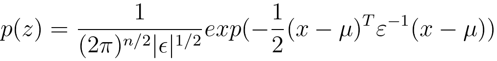
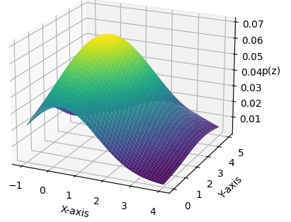
In Gaussian Discriminant Analysis (GDA), we can ssume that the feature variables (x) are continuous and belong to the n-dimensional real space, denoted as ℝⁿ. Typically, you include an additional feature with a constant value (1) to account for bias. If they're dropping this convention, then x is considered to be in ℝⁿ rather than ℝⁿ + 1. The key assumption in Gaussian Discriminant Analysis is that the conditional probability distribution of feature variables P(x|y) is Gaussian (normal) for each class y. In other words, the feature variables for each class follow a Gaussian distribution. The expected value of z can be given by the Gaussian distribution for z, where, μ represents the mean vector ( µ ∈ Rn) of the Gaussian distribution for z. represents the covariance matrix (Σ ∈ Sn++). For instance for is the random variable for which you are calculating the probability density. is the dimensionality of the random variable . Both μ and σ are two-dimensional (2D), matching the dimensionality of z. E[z] = μ ------------------------------- [3848b] Covariance of Z, which typically represents how the components of the random variable z are correlated, where, E[z] = Ez for simplified notation. A vector-valued random variable X =[X1, X2, · · · ,Xn]T has a probability of density function, which is given by Multivariate Gaussian Distribution [1], The right-hand side of the equation is a mathematical expression for the probability density of the random variable with respect to the parameters , , and . With defined parameters n = 2, ε = [[2, 1], [1, 3]], and μ = [1, 2] (with with components and ), to represent the dimension, covariance matrix, and mean vector of the distribution, the probability of density function is plotted in Figure 3848a. The probability density function is defined over a two-dimensional space, and the X-axis and Y-axis correspond to the values of in those two dimensions. In Figure 3848a (a), the contour lines represent the values of the probability density function at different points in this two-dimensional space. Note that there are no specific X-axis and Y-axis on the right-hand side of Equation 3848e. Instead, this equation represents the probability density as a function of the random variable , which you can evaluate for different values of to obtain the probability density at those points. The X-axis and Y-axis are only used when visualizing the function in a plot. These parameters , , and define the shape, location, and scale of the PDF, and thus control the mean and the variance of this density. Here, the mean is a vector , which determines the center of the distribution in the multi-dimensional space. The variance related is a covariance matrix, which contains information about the variances and covariances of the different components of the random variable and describes how spread out or concentrated the data is in different dimensions.
(a)
(b)
(c)
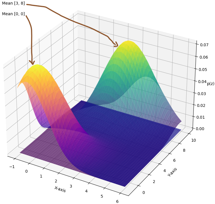
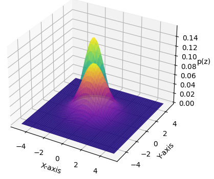
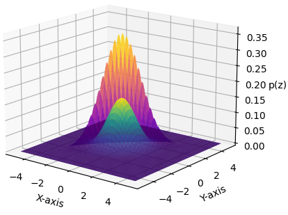
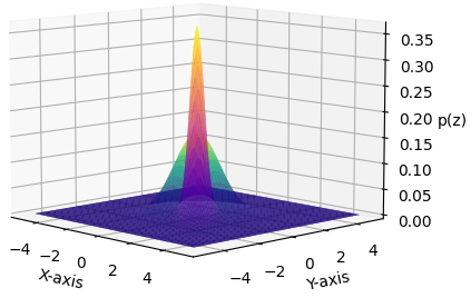
Figure 3848b shows the probability of density function in 3D with = [[1, 0], [0, 1]] and [[1.5, 0], [0, 1.5]], with = [[1, 0], [0, 1]] and [[1, 0.9] and with = [[1, 0], [0, 1]] and [[1, -0.5], [-0.5, 1]]. When the covariance is reduced, then the spread of the Gaussian density is reduced, and the distribution is taller because the area under the curve must be integrated to 1. Furthermore, changing μ can shift the center of the Gaussian density around.
(a)
(b)
(c)
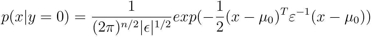
Based on Equation 3848e, in GDA model, p(x|y=0) and p(x|y=1) can be given by Gaussian distribution, Equations 3848f and 3848g describe conditional probability density functions. These equations are commonly associated with Gaussian (or normal) distributions in classification problem or Bayesian statistics:
In machine learning, with Gaussian distribution, the prior distribution of θ can be given by, This is a Gaussian (Normal) distribution with mean zero and a covariance matrix of τ2I, where I is the identity matrix. This is a common choice for the prior distribution in Bayesian regularization in machine learning. In a classification context, these equations are used for modeling the conditional probability of an input x belonging to class 0 (y=0) or class 1 (y=1) when you assume that the data follows a Gaussian distribution with class-specific mean values (μ₀ and μ₁) and a shared covariance matrix (ε). Based on logistic regression, we have, where, p(y): This represents the probability of a binary random variable y taking on a specific value, which can be either 0 or 1. y is the Bernoulli random variable. This is the random variable, which can take on one of two values, either 0 or 1. Φ = p(y=1), which is a parameter of the Bernoulli distribution, and it represents the probability of success or the probability that y equals 1. (1-Φ): This is the probability of failure or the probability that y equals 0. Since there are only two possible outcomes (0 and 1), the sum of φ and (1-Φ) must equal 1. µ0 ∈ Rn, µ1 ∈ Rn, ϵ ∈ Rn x n, and Φ ∈ Rn. The probability distribution function given in Equation 3848h shows the probability mass function for a Bernoulli distribution. Equation 3848h calculates the probability of y taking on a particular value based on the parameter Φ. When y is 1, the probability is Φ, and when y is 0, the probability is (1-Φ). This is a fundamental model for situations where you have binary outcomes, like heads or tails in a coin toss, success or failure in a trial, etc. A training set in machine learning can be given by, Some other notations can be used in Maximum Likelihood Estimation (MLE) as well. Multiple parameter estimation is given by, µ0 can be given by, where,
µ1 can be given by, On the other hand, we have, where, is the difference between the data point x(i) and its corresponding mean μy(i). This is a vector subtraction, resulting in a vector that represents the deviation of 'x^{(i)}' from its mean. GDA is particularly useful when the data is normally distributed and the class-conditional distributions have different covariances. When GDA is used for prediction in supervised machine learning tasks, the GDA process is below:
a. For a given input feature vector, calculate the likelihood of the data given each class's Gaussian distribution. This involves computing the probability density function (PDF) of the data for each class. In the step of making predictions, when we assign the input data point to a class based on the posterior probabilities calculated for each class, we can use the equation below, where, represents the posterior probability of class given the input data point . is the likelihood of the data given that it belongs to class . is the prior probability of class . In this step, you are comparing the posterior probabilities for each class, and the class with the highest posterior probability is the one to which you assign the input data point. The equation (Equation 3848p) is part of the decision-making process in this step, helping you determine the class with the maximum posterior probability. b. Multiply the likelihood by the prior probability of the class (the proportion of the training data that belongs to that class). c. Normalize the results to obtain posterior probabilities for each class. This can be done using Bayes' theorem. d. Assign the input data point to the class with the highest posterior probability. Note that it's a common simplification in many classification tasks to treat as a constant across all classes when you're only interested in finding the class with the maximum posterior probability, because:
Table 3848. Applications of Gaussian Discriminant Analysis.
============================================
[1] Chuong B. Do, The Multivariate Gaussian Distribution, 2008.
|
||||||||
| ================================================================================= | ||||||||
|
|
||||||||

 ------- [3848e]
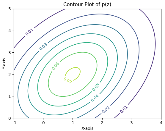
 ------- [3848f]
 ----- [3848g]
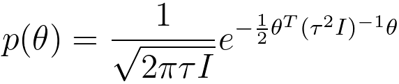 ------------------- [3848gb]
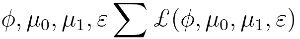 ----------------------------------- [3848j]
 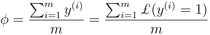 ----------------------------------- [3848k]
 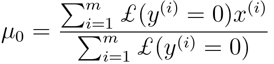 ----------------------------------- [3848l]
 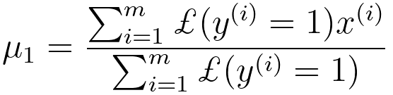 ----------------------------------- [3848m]
 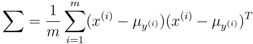 ----------------------------------- [3848n]
 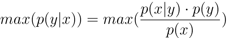 ----------------------------------- [3848p]