Generalization Risk/Generalization Error versus Empirical Risk
- Python Automation and Machine Learning for ICs - - An Online Book - |
|||||||||||||||||||||||||||
| Python Automation and Machine Learning for ICs http://www.globalsino.com/ICs/ | |||||||||||||||||||||||||||
| Chapter/Index: Introduction | A | B | C | D | E | F | G | H | I | J | K | L | M | N | O | P | Q | R | S | T | U | V | W | X | Y | Z | Appendix | |||||||||||||||||||||||||||
================================================================================= Table 3760. Generalization risk versus empirical risk.
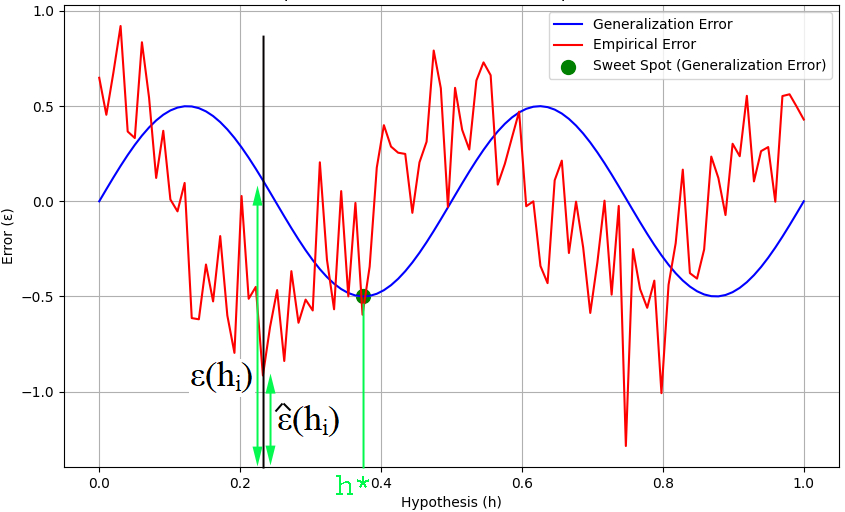
Figure 3760a shows dependence of both generalization and empirical error on hypothesis. The ε(hi) and ε^(hi) at hypothesis hi has been marked in the figure. The expected value of ε^(hi) is given by, E[ε^(hi)] = ε(hi) ---------------------------------- [3760a]
Figure 3760a. Dependence of both generalization and empirical error on hypothesis. (code) The sweet spot gives the h*, which is the best h in a class. Now, we apply the Hoeffding Inequality, then we can get, where,
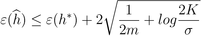
This inequality provides a bound on the probability that the absolute difference between the empirical error and the generalization error exceeds a certain value . It is a key result in statistical learning theory and is often used to analyze the generalization performance of learning algorithms. As we increase the sample size m, then the righ side of Inequality 3760b becomes very small. Therefore, the empirical error will be around the generalization error. That means, with the increase of the sample size, the probability that the absolute difference between the empirical error and the generalization error is greater than γ will be very small because it is bounded by the right side of Inequality 3760b. However, in practice, we do not fix hi before the training. Instead, we have data first and then find the correct hi for the data. Then, we find a bound for all hi. This process is called uniform convergence. Uniform convergence helps us obtain the empirical risk converges uniformly to the expected risk as we increase the amount of training data. In the process above, we got the bound for a specific hi. Next step is that we want to get Union Bound across all hi. The union bound is a way to combine the probabilities or bounds associated with multiple events. This will be two different possible cases. One is a case of a finite hypothesis class, and the other is infinite hypothesis class. Then, the next step, based on Figure 3760a, is to get (at hi), ε(h^) ≤ ε^(h^) + ϒ ------------------------------------------ [3760c] ≤ ε^(h*) + σ ------------------------------------------ [3760d] ≤ ε(h*) + 2ϒ ------------------------------------------ [3760e] That is, based on the probabiligy for 1 - σ with the training size m in Inequality 3760b, we can have, For VC (Vapnik-Chervonenkis) classes, we have, where, : This is the Vapnik-Chervonenkis dimension of the hypothesis space , which is a measure of the capacity or complexity of the hypothesis space. : This represents the confidence level. The part of "O square root" represents an upper bound on the difference between the expected true error of ℎ^ and ℎ*, and it is derived based on the Vapnik-Chervonenkis dimension and the size of the training dataset. ============================================
|
|||||||||||||||||||||||||||
| ================================================================================= | |||||||||||||||||||||||||||
|
|
|||||||||||||||||||||||||||
 ------------------------------------- [3760f]
 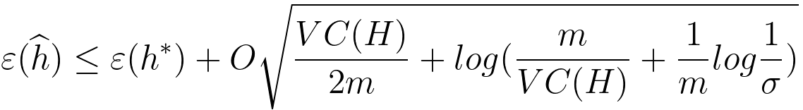 ------------------------------------- [3760g]