=================================================================================

The Grid World Navigation problem is a classic reinforcement learning task commonly used to study and test algorithms in the field of machine learning. The task involves an agent navigating through a grid-like environment to reach a goal while avoiding obstacles.

The key components of the problem are:

1. Environment: The environment is represented as a grid, where each cell can be either empty, containing an obstacle, or the goal.

2. Agent: The agent is the entity that moves within the grid. The goal of the agent is to learn a policy (π) that allows it to navigate from a starting position to the goal while avoiding obstacles.

3. Actions (A): The agent can take actions to move in different directions within the grid. Common actions include moving up, down, left, or right.

4. Rewards (R): The agent receives rewards based on its actions. Typically, the agent receives a positive reward for reaching the goal and a negative reward for colliding with obstacles. The goal is to learn a policy that maximizes the cumulative reward over time. The range of rewards in reinforcement learning can vary depending on the specific application and problem formulation. In many cases, rewards are real numbers and can span a wide range, including positive, negative, or zero values. The key is to define the rewards in a way that provides meaningful feedback to the learning agent. Some common conventions for reward ranges are:

1. Positive Rewards: Positive rewards are often used to reinforce desired behaviors. For example, reaching a goal state might be associated with a positive reward, such as +1.

2. Negative Rewards (Penalties): Negative rewards, or penalties, are used to discourage undesired behaviors. Colliding with obstacles or taking inefficient paths might result in negative rewards, such as -1.

3. Zero Reward: Zero is often used as a neutral or baseline reward. Some actions or states might have a neutral impact on the agent's overall performance.

4. Unbounded Rewards: In some scenarios, rewards may have an unbounded range, meaning they can take any real value. This is common when the magnitude of the reward is crucial for conveying the significance of an outcome.

5. Learning Objective: The learning objective is to train the agent to learn an optimal or near-optimal policy for navigating the grid. This is often done using reinforcement learning algorithms, where the agent explores the environment, receives feedback in the form of rewards, and adjusts its policy to improve performance.

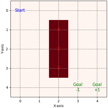
5.a. In Value Iteration, the agent learns a policy, a mapping from state to action, guiding its decisions at each state. However, our approach diverges by initially utilizing Value Iteration to learn a mapping of state to value, estimating rewards. Subsequently, the agent selects actions at each state based on these reward estimates, aiming to maximize cumulative rewards by choosing the actions associated with the highest estimated rewards.

Researchers and practitioners use the Grid World Navigation problem as a simplified testbed to develop and evaluate reinforcement learning algorithms before applying them to more complex real-world tasks. It serves as a foundation for understanding concepts such as state, action, reward, and the exploration-exploitation trade-off in reinforcement learning.

As an example, the guideline of the navigation is straightforward: Your agent or robot commences its journey from the top-left corner (indicated as the 'start' position) and concludes at either Goal +1 or Goal -1, as shown in Figure 3683a, representing the corresponding reward. At each step, the agent has four feasible actions, namely up, down, left, and right. The red blocks signify impenetrable walls, barring the agent from passing through them. Initially, our implementation assumes determinism in actions—each action leads the agent precisely to its intended destination. For instance, if the agent opts for the "up" action at coordinates (2, 0), it will unfailingly land at (1, 0) rather than at (2, 1) or any other location. However, in the event of encountering a wall, the agent remains stationary at its current position.

Figure 3683a. Grid world navigation (code).

Initially, the agent initializes the estimated values of all states V(S)) to zero,

          ------------------------- [3683a]

The agent explores the environment by randomly moving within the grid. Initially, with no knowledge, the agent endures failures, but it learns from each iteration. An update rule commonly, which is associated with the update step for the value of a state S_t​ , used in reinforcement learning and temporal difference learning is,

          ------------------------- [3683b]

where,

• V(S_t) is the current estimated value of state S_t.
• V(S_t+1) is the estimated value of the next state S_t+1.
• α is the learning rate, a constant parameter between 0 and 1 that determines the step size of the update.
• [V(S_t+1) -V(S_t)] is the temporal difference, representing the difference between the estimated values of the current state and the next state.

The corresponding steps and their corresponding parameter updates are:

          S₀

          a₀

          S₁, ~ P(S₀, a₀)

          R(S₀) + ϒR(S₁)

          a₁

          S₂, ~ P(S₁, a₁)

          ...

          R(S₀) + ϒR(S₁) + ϒ²R(S₂) + ...

The update rule signifies that the current estimate V(S_t) is adjusted by a fraction α of the temporal difference [V(S_t+1)-V(S_t)]. This adjustment helps the agent update its value estimates based on the new information obtained from experiencing the transition from state S_t​ to S_t+1. The learning rate α influences the weight given to the new information in the update. In the navigation completion, The game resets when the agent reaches the end with a reward of +1 or -1, and rewards propagate backward, updating the estimated values of states encountered during the navigation.

The agent evolves from an initial state of no knowledge, exploring and learning from failures. The update formula reflects how the estimated value of a state is adjusted based on the new information acquired during each iteration of game playing, influenced by the learning rate (α). For example, if the agent moves from state S₁​ to S₂​ with a reward of 1, the new estimate of S₁​ is calculated as S₁​ + α(S₂​ − S₁).

We can use a stochastic version to incorporate probabilities into the reinforcement learning update rule. In a simple case where the agent can take one of four actions (up, down, left, right) with equal probability. The update rule in this stochastic case would be,

          ----------------- [3683c]

where:

• R_t+1​ is the reward obtained after taking action a at state S_t.
• γ is the discount factor (a constant between 0 and 1).
• max_a'​ V(S_t+1, a') represents the maximum expected future reward at the next state S_t+1.

Assuming the agent chooses each action with equal probability. In a stochastic environment, the probability of transitioning from state S_t​ to state S_t+1​ with action a can be denoted as P(S_t+1|S_t, a). If each action is equally likely, the probabilities can be set as follows,

          ---------- [3683d]

Then, the update rule becomes,

          ----------------- [3683e]

This formula considers the equal probability of taking each action. In a more complex scenario, where action probabilities are different, these probabilities would be incorporated accordingly.

If the agent has a 20% chance of moving in a different direction when heading north (or any other direction), we then need to introduce this stochasticity into the update equation. We can modify the equation to account for the probabilities associated with each action. Assuming the agent has an 80% chance of moving in the intended direction and a 20% chance of moving in a different direction, the update equation becomes more complex. Let's denote the intended action (e.g., moving north) as a and the alternative actions (e.g., moving in other directions) as a'. The update equation with the stochasticity will be changed to,

     ------ [3683f]

where:

• 4/5​ is the probability of taking the intended action.
• 1/5​ is the probability of taking an alternative action.
• Average_a'V(S_t+1​, a') represents the average value over all alternative actions.

This modification assumes an equal probability distribution among the alternative actions when the agent deviates from the intended direction. The probabilities and the update equation need to be adjusted accordingly if the actual probabilities are different.

Based on reinforcement learning, if we consider the possibility of unintended movements due to uncertainties or stochasticity in the environment, we can introduce probabilities for each possible action. Let's assume that there's a 20% chance of going in the intended direction (down) and a 20% chance of going in each of the other three directions (up, left, right). In this case, the equations would involve calculating the expected value for each possible outcome. The equations for moving down, up, left, and right from position (3, 2) are as follows:

1. Moving Down (Intended Direction):

   • (i', j') for down: (4, 2).
   • Immediate Reward: R(i', j') = reward(4, 2, goal).
   • Expected Future Value: Expected Future Value = γV(i', j').
   • Total Expected Value: Expected Value_down = R(i', j') + Expected Future Value
2. Moving Up (Unintended Direction):
   • (i', j') for up: (2, 2).
   • Immediate Reward: R(i', j') = reward(2, 2, goal).
   • Expected Future Value: Expected Future Value = γV(i', j').
   • Total Expected Value: Expected Value_up = R(i', j') + Expected Future Value
3. Moving Left (Unintended Direction):
   • (i', j') for left: (3, 1)
   • Immediate Reward: R(i', j') = reward(3, 1, goal)
   • Expected Future Value: Expected Future Value = γV(i', j').
   • Total Expected Value: Expected Value_left = R(i', j') + Expected Future Value
4. Moving Right (Unintended Direction):
   • (i', j') for right: (3, 3)
   • Immediate Reward: R(i', j') = reward(3, 3, goal)
   • Expected Future Value: Expected Future Value = γV(i', j').
   • Total Expected Value: Expected Value_right = R(i', j') + Expected Future Value

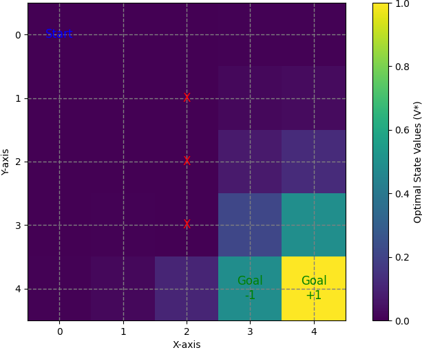
To combine the equations for the different directions (down, up, left, right) and represent the update for the state value V(3, 2), we can use a weighted sum of the expected values for each direction. Assuming a 20% probability for each direction, the update V(3, 2) can be expressed as follows:

        
                          ------ [3683g]

where,

Expected Value_stay represents the case where the agent stays in the current position. The probabilities (0.2 for each direction) indicate the likelihood of each action occurring.

Figure 3683b shows the optimal value at each state.

Figure 3683b. Optimal value at each state (code).

Insert the values in Figure 3683b into Equation 3683g, then we have,

        V(3,2) = 0.2*0.6 + 0.2*0.01 + 0.2*0.01 + 0.2*0.4 + 0.2*0.25 = 0.29 ----------------- [3683h]

============================================