=================================================================================

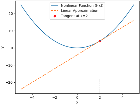
Linearization is a process of approximating a nonlinear model with a linear one around a specific operating point. This is often done to simplify the analysis and design of control strategies, such as applying linear control techniques like the Linear Quadratic Regulator (LQR). The linearization process involves finding the first-order Taylor series expansion of the nonlinear model. Figure 3661a shows an example of linearization. The grey dash line indicates the selected operating point mentioned below.

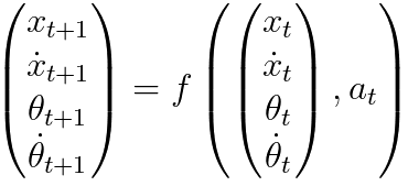
Figure 3661a. Linearization.

The general steps to linearize a nonlinear model are:

i) Understand the Nonlinear Equation:

For instance, in the non-linear mode of reinforcement learning (RL), we can have,

           ------------------------ [3661a]

           ------------------------ [3661b]

Here, the derivatives can be different velocities.    

ii) Select an Operating Point:

        Choose an operating point around which you want to linearize the model. This is the point at which you'll evaluate the nonlinear equations and compute the linearization.

        For the RL case, we select an point .

iii) Define State and Input Variables:

         Identify the state variables (x) and input variables (u) in your nonlinear model. These are the variables that describe the system's state and the control inputs. 

iv) Write Down Nonlinear Equations:

         Express the nonlinear dynamic equations of the system. These equations might be in the form of differential equations or discrete-time update equations, depending on the nature of the system. 

v)  Compute Partial Derivatives:

         Compute the partial derivatives of the nonlinear equations with respect to the state variables and control inputs. These derivatives represent the sensitivity of the system's dynamics to changes in the state and control input. 

vi) Evaluate Derivatives at the Operating Point:

         Substitute the values of the state and control input at the chosen operating point into the partial derivatives. This gives you the linearization evaluated at the operating point.  

 vii) Form Linearized Equations:

         Combine the linearized terms to form a set of linearized equations that describe the system's dynamics around the operating point. The linearized equations are typically in the form of for continuous-time systems or x_k+1 = Ax_k+ Bu_k for discrete-time systems. 

         For the RL case,  we then have,

           ------------------------ [3661c]

where,

         S_t+1 represents the next state of the system. 

           represents the Jacobian matrix of the nonlinear function f evaluated at the operating point . The Jacobian matrix contains the partial derivatives of each component of f with respect to each state variable. It characterizes the local linear behavior of the system around the operating point. 

           represents the sum of the current state S_t and the operating point . This term is used to model the perturbation from the operating point. 

           is the evaluation of the nonlinear function f at the operating point . It represents the baseline behavior of the system without considering deviations from the operating point.

Equation 3661c is an approximation of the state transition in a nonlinear system, linearized around an operating point. 

When we consider both state s and action a, then Equation 3661c becomes,  

           ------------------ [3661d]

The overall equation is an approximation that combines both the local linear behavior (given by the Jacobian term) and the baseline behavior (given by the function evaluation term). The linearization is useful for analyzing the system's behavior near the operating point and for designing control strategies, especially when linear control methods such as the Linear Quadratic Regulator (LQR) are applied. 

============================================