=================================================================================

In principal component analysis (PCA), the objective is often to reduce the dimensionality of the data while retaining as much variance as possible. By selecting the eigenvectors with the largest eigenvalues (i.e., the top eigenvectors), we are prioritizing the components that capture the most significant sources of variation in the dataset. 

The sum of the variances explained by all the principal components in PCA is 100%. In PCA, the principal components are ordered by the amount of variance they explain in the data. The first principal component explains the most variance, the second principal component explains the second most variance, and so on. The sum of the variances explained by all the principal components is equal to the total variance in the original data. Therefore, it's common to express the variance explained by each principal component as a percentage of the total variance, and the sum of these percentages will be 100%. This property is often used to determine how many principal components to retain in a PCA analysis. We might decide to keep enough principal components to explain a certain percentage of the total variance, such as 90% or 95%.

The steps on how to calculate PCA are shown below (in the example below, given a dataset X with n observations and p features): 

• Standardize the Data: If the data is not on the same scale, it's important to standardize it so that each feature contributes equally to the analysis. To standardize the data, subtract the mean of each feature and divide by its standard deviation. 

 --------------------------------- [3461a]

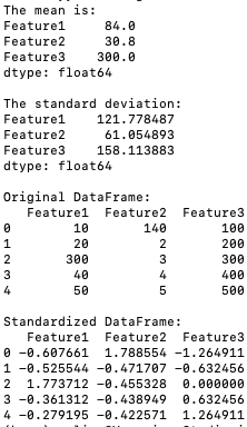
The program below standardizes the data (code):  

 

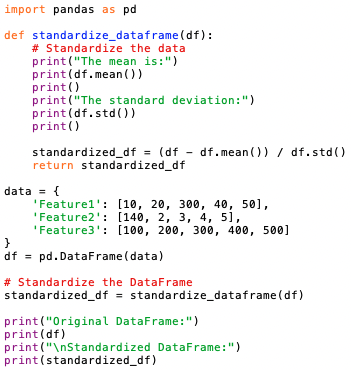
Output:

The standardization formula (X - mean) / std is applied to each column of the DataFrame using pandas' broadcasting functionality. The standardized data is mean-centered and scaled to unit variance.

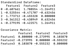
• Compute the Covariance Matrix: The covariance matrix summarizes the relationships between all pairs of features in the dataset. It is calculated by multiplying the transpose of the standardized data matrix by itself and dividing by the number of observations. 
  

 --------------------------------- [3461b]

The program below computes the covariance matrix (code):

 

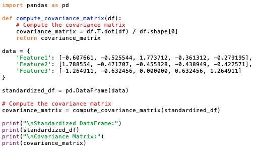
Output:

This code computes the covariance matrix using the transpose of the standardized data matrix multiplied by the standardized data matrix itself, divided by the number of observations.

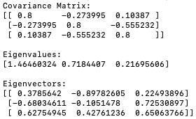
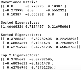
• Calculate the Eigenvectors and Eigenvalues: Eigenvectors and eigenvalues are the key components of PCA. Eigenvectors represent the directions (or components) of the data that explain the most variance, while eigenvalues represent the magnitude of variance along those directions. We can compute them by performing an eigendecomposition on the covariance matrix. 
  

 --------------------------------- [3461c]

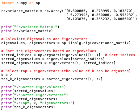
The program below calculates the eigenvectors and eigenvalues (code):

 

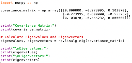
Output: 

Eigenvalues represent the amount of variance explained by their corresponding eigenvectors. Eigenvectors associated with larger eigenvalues explain more variance in the data. When we sort the eigenvalues in descending order, we essentially rank the eigenvectors by the amount of the variance of the original data they capture. Eigenvectors corresponding to higher eigenvalues capture more variance and are therefore considered more important in representing the data's structure. By selecting the eigenvectors with the largest eigenvalues (i.e., the top eigenvectors), we prioritize capturing the most significant sources of variation in the original dataset. These top eigenvectors represent the principal components that best explain the variability present in the data's structure.

• Select Principal Components: Sort the eigenvectors by their corresponding eigenvalues in descending order. These sorted eigenvectors are called principal components. Typically, we will select the top k eigenvectors based on the explained variance we desire (e.g., 95%). 

  The program below calculates the eigenvectors and eigenvalues (code):

   

  Output:



• Transform the Data: Finally, we can transform the original data into the new feature space defined by the selected principal components. This is achieved by multiplying the standardized data matrix by the matrix of selected eigenvectors. 
  

 --------------------------------- [3461d]

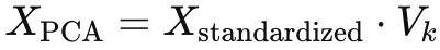
The program below multiplies the standardized data matrix by the matrix of selected eigenvectors  (code):

 

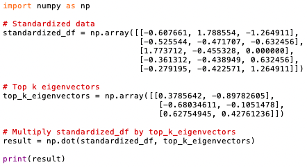
Output: 

 

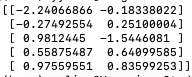
The resulting matrix "result" contains the transformed data after the dimensionality reduction using the selected eigenvectors as principal components. The positive and negative numbers represent the projections of the original data points onto the principal components (eigenvectors):

• Magnitude of Values: The magnitude of the values indicates the relative importance of the principal components in representing the original data. Larger absolute values suggest that the corresponding principal component contributes more significantly to the representation of the data point. 

• Sign of Values: The sign of the values (positive or negative) indicates the direction of the projection along the principal component axis. Positive values indicate a projection in the direction of the positive axis of the principal component, while negative values indicate a projection in the opposite direction.

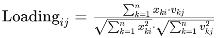
• Calculate Loadings: The loadings can be calculated as the correlation between the original variables and the principal components. We can compute this using the correlation coefficient formula:

   --------------------------------- [3461e]

  where,

  • x_ki represents the standardized value of the original variable i in observation k. 

  • v_kj represents the j-th element of the k-th eigenvector (principal component). 

  • n is the number of observations. 

  • The denominator normalizes the loading to account for the scaling of the original variables and the principal components. 

  The loadings indicate the strength and direction of the relationship between each original variable and each principal component. Larger absolute values of loadings suggest stronger relationships. Positive loadings indicate positive correlations, while negative loadings indicate negative correlations.

  The program below calculates the loadings  (code):

   

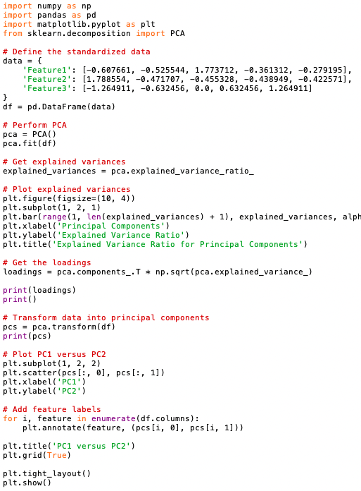
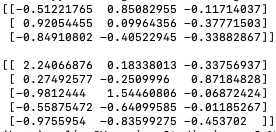
  Output:

  

   

  The library that implements PCA with Equation 3461e is scikit-learn (or sklearn), namely "from sklearn.decomposition import PCA" in the code.

  The loadings indicate the correlation between the original variables (features) and the principal components. Positive and negative loadings represent the direction and strength of this correlation. 

  • Positive Loadings: A positive loading indicates a positive correlation between the original variable and the principal component. This means that as the original variable increases, the corresponding principal component also increases. In other words, high values of the original variable are associated with high values of the principal component, and vice versa. 

  • Negative Loadings: A negative loading indicates a negative correlation between the original variable and the principal component. This means that as the original variable increases, the corresponding principal component decreases, and vice versa. High values of the original variable are associated with low values of the principal component, and vice versa. 

  The magnitude of the loading indicates the strength of the correlation. Larger absolute values indicate stronger correlations, while values closer to zero indicate weaker correlations.

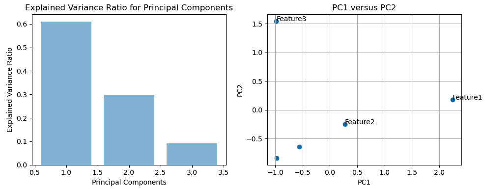
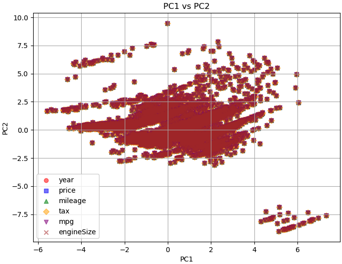
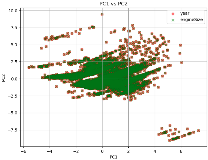
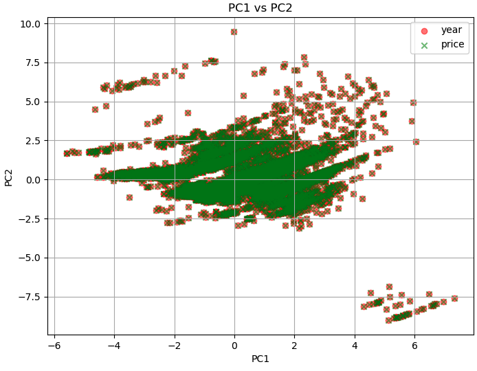
  In PCA, the principal components are derived from linear combinations of the original features. The first principal component (PC1) captures the direction of maximum variance in the data, followed by PC2, which captures the direction of maximum variance orthogonal to PC1, and so on. In the plot of PC1 versus PC2, the data points that are similar in terms of those features will likely cluster together in the PC1 versus PC2 plot. Such similar features being grouped together on the PC1 versus PC2 plot is a magic of PCA.
  
  

============================================

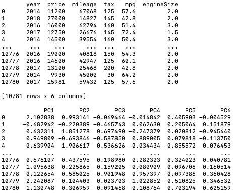
Principal component analysis for cars (code) with input data:

         

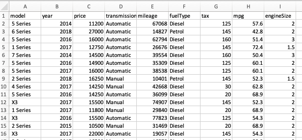
Output:         

         

         

         

         

============================================