Table 3383. Comparison between Naive Bayes algorithms and Bayesian machine learning techniques.
| |
Naive Bayes algorithms |
Bayesian machine learning techniques |
| Overview |
- Naive Bayes is a specific type of classification algorithm based on Bayes' Theorem with the assumption of independence among predictors. It is called "naive" because it assumes that the presence of a particular feature in a class is unrelated to the presence of any other feature.
- It is primarily used for classification tasks, such as spam email detection or document categorization. Despite its simplicity and the strong independence assumption, Naive Bayes can perform very well and is particularly efficient with large datasets.
|
- Bayesian techniques in ML encompass a much broader range of applications than Naive Bayes. These techniques use Bayesian inference as a methodological basis, which involves updating the probability estimate for a hypothesis as more evidence or information becomes available.
- Bayesian methods are used in various ML tasks beyond classification, including regression, clustering, and optimization. These methods allow for incorporating prior knowledge into models, handling missing data, making probabilistic predictions, and modeling complex systems.
|
Bayes’ Theorem
(overlap 1) |
Both Naive Bayes algorithms and broader Bayesian machine learning techniques are grounded in Bayes' Theorem, which relates the conditional and marginal probabilities of random events. Bayes' Theorem is used to update the probability estimate for a hypothesis as evidence is added. |
Probabilistic Approach
(overlap 2) |
Both approaches inherently take a probabilistic view of data and predictions. This means they both provide outputs in terms of probabilities, giving not only predictions but also a measure of certainty or uncertainty about these predictions. |
Incorporation of Prior Knowledge
(overlap 3) |
Both methods can incorporate prior knowledge into the model. In Naive Bayes, this might be done through the prior probability distributions assigned to different classes. In broader Bayesian modeling, prior distributions can be more complex and nuanced, influencing various parameters of the model. |
| Main difference |
Naive Bayes is limited by its assumption of feature independence within classes, which simplifies computation but can limit accuracy when this assumption does not hold. It's primarily used for classification tasks. |
Bayesian Machine Learning Techniques encompass a wider array of methods and are used for various tasks beyond classification, including regression, clustering, and sequential data analysis. These techniques are more flexible in handling complex and interdependent data structures, often using sophisticated models like Bayesian networks, Gaussian processes, or hierarchical Bayesian models. |
| Foundational Principles |
- Based on Bayes’ Theorem.
- Assumes that all predictors (features) are independent of each other given the class.
- Uses simple probability models for each class and feature based on the training data.
|
- Based on Bayes’ Theorem but typically involves more complex probabilistic models.
- Does not necessarily assume independence among features.
- Often uses prior distributions to incorporate existing knowledge before observing the data, and updates beliefs with posterior distributions after considering the data.
|
| Model Complexity |
- Generally simpler and more computationally efficient.
- Due to its simplicity and the independence assumption, it can be outperformed by more sophisticated models on complex tasks.
- Easy to implement and fast to train.
|
- Can be very complex, involving layered models and dependencies.
- Computationally intensive, especially as model complexity increases.
- Flexible in handling a wide range of problems, including those where relationships among data points are important.
|
| Applicability |
- Mainly used for classification tasks.
- Effective in scenarios where the independence assumption holds reasonably well or when the data dimensionality is high relative to the sample size.
- Popular in spam detection, sentiment analysis, and document classification.
|
- Applicable to a broad set of machine learning tasks, including classification, regression, clustering, and time-series analysis.
- Used in areas requiring robust uncertainty estimation and risk management, like financial forecasting, clinical trials analysis, and adaptive testing systems.
|
| Typical Use Cases |
- Often used when the model speed is critical and the data set is large.
- Works well with text data, especially for applications like email filtering and real-time prediction.
|
- Ideal for problems where model interpretability and uncertainty quantification are important.
- Used in scientific research for hypothesis testing, in robotics for decision making under uncertainty, and in marketing analytics for customer segmentation.
|
| Handling of Data and Uncertainty |
- Handles missing data by ignoring the missing values during model building and prediction.
- Provides probabilistic outputs, offering a measure of certainty about predictions, which can be a significant advantage over non-probabilistic classifiers.
|
- Typically better at handling missing data and incorporating uncertainty in a more systematic and principled way.
- Often uses Monte Carlo methods or variational inference to approximate complex posteriors, providing detailed insights into data uncertainty and model predictions.
|
| Scalability |
Highly scalable due to its simplicity, making it suitable for very large datasets and real-time applications. |
Scalability can be an issue, especially with very complex models. Advanced computational techniques like Markov Chain Monte Carlo (MCMC) are often necessary but computationally costly. |
Bayes’ Theorem
(overlap 4) |
The general form of Bayes' Theorem is:
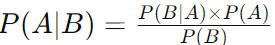
where:
- P(A∣B) is the posterior probability of hypothesis A given the data B.
- P(B∣A) is the likelihood, which is the probability of observing the data B given that hypothesis A is true.
- P(A) is the prior probability of hypothesis A being true (before considering the data B).
- P(B) is the evidence, the total probability of observing the data B.
|
| Equations |
Naive Bayes simplifies Bayes’ Theorem by assuming that the features (variables) in the data are conditionally independent given the outcome. This assumption allows for the straightforward calculation of the likelihood by multiplying the probabilities of each individual feature. For a classification task with features X = (x1, x2, ..., xn) and class variable C, the Naive Bayes formula becomes:
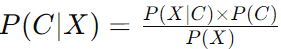
Where,
P(X∣C), under the independence assumption, simplifies to:

Thus, the classifier can be written as:

We typically ignore P(X) in the denominator during computation since it does not depend on C and we're interested in finding the class C that maximizes P(C∣X). |
In broader Bayesian models, the approach becomes more complex and nuanced. These models do not typically assume independence among features and can accommodate complex relationships and hierarchical structures. The general equation using Bayes’ Theorem in Bayesian models is:
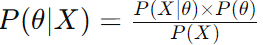
where:
- θ represents the parameters or hypotheses we're trying to learn.
- P(θ∣X) is the posterior distribution of the parameters given the data.
- P(X∣θ) is the likelihood of the data given the parameters.
- P(θ) is the prior distribution of the parameters.
- P(X) again serves as the normalizing constant.
In practice, Bayesian models often involve:
- Integrating out parameters using numerical methods when the denominator cannot be analytically calculated.
- Using Markov Chain Monte Carlo (MCMC), Variational Inference, or other computational techniques to estimate the posterior distribution P(θ∣X) when direct calculation is infeasible.
|
| Assumption |
Naive Bayes assumes feature independence. |
Feature independence is not assumed in general Bayesian models. |
| Computational Complexity |
Naive Bayes is computationally simpler and faster due to its assumptions. |
Bayesian methods can be computationally intensive. |
| Flexibility |
Naive Bayes cannot model complex dependencies. |
Bayesian models are more flexible and can model complex dependencies. |
| Application Scope |
Naive Bayes is primarily used for classification. |
Bayesian techniques span classification, regression, clustering, and more. |
| Python libraries |
Scikit-learn (sklearn) is one of the most popular machine learning libraries in Python. It provides several types of Naive Bayes classifiers, including Gaussian Naive Bayes, Multinomial Naive Bayes, and Bernoulli Naive Bayes. It's well-suited for those new to machine learning, as well as for those who need to implement standard ML algorithms efficiently.
Usage Example:
from sklearn.naive_bayes import GaussianNB
model = GaussianNB()
model.fit(X_train, y_train)
|
A couple of Python libraries can be used for Bayesian machine learning.
PyMC3 is a library designed for building Bayesian models and making Bayesian inference. It uses Theano to compute gradients via automatic differentiation and supports various MCMC sampling methods.
Usage Example:
import pymc3 as pm
with pm.Model() as model:
# Model definition
pass
Stan is a powerful tool for performing Bayesian data analysis using probabilistic programming. PyStan provides a Python interface to Stan, enabling the development and diagnostic of sophisticated statistical models.
Usage Example:
import pystan
model_code = 'parameters {real y;} model {y ~ normal(0,1);}'
model = pystan.StanModel(model_code=model_code)
fit = model.sampling()
TensorFlow Probability is a library for probabilistic reasoning and statistical analysis in TensorFlow. It supports a wide range of Bayesian and probabilistic models and is useful for those who are already using TensorFlow for other types of machine learning.
Usage Example:
import tensorflow_probability as tfp
tfd = tfp.distributions
# Define a normal distribution
normal = tfd.Normal(loc=0., scale=1.)
ArviZ is an open-source library for exploratory analysis of Bayesian models. It is compatible with all of the above frameworks and provides a unifying interface for doing inference data diagnostics and model criticism.
Usage Example:
import arviz as az
az.plot_trace(fit) # Where fit is from PyMC3, Stan, or another inference engine
|
| General applications |
Naive Bayes is particularly popular for classification tasks where the dimensionality of the input data is high relative to the dataset size. Common applications include:
- Email Spam Detection: Classifying emails as spam or not spam based on the presence of certain keywords.
- Sentiment Analysis: Determining the sentiment expressed in texts, such as reviews or social media posts, by classifying the texts as positive, negative, or neutral.
- Document Classification: Automatically categorizing documents into predefined topics based on their content, used in digital libraries and information retrieval systems.
- Disease Prediction: Classifying patients as having a particular disease or not, based on symptoms and test results, used in medical diagnostics.
- Fraud Detection: Identifying fraudulent activities, like credit card fraud, by analyzing transaction patterns.
|
Bayesian methods are used in more diverse and complex scenarios, including:
-
Predictive Modeling:
- Weather Forecasting: Using historical data to predict future weather conditions.
- Stock Market Analysis: Forecasting stock prices and market trends based on historical data and economic indicators.
- Robotics:
- Navigation and Mapping: Robots use Bayesian techniques to build maps of environments and navigate through them using sensors and previous knowledge.
- Natural Language Processing:
- Machine Translation: Translating text or speech from one language to another using models that incorporate the likelihood of sequence of words.
- Information Extraction: Identifying specific pieces of information, such as named entities, from large text corpora.
- Bioinformatics:
- Genetic Association Studies: Identifying associations between genetic variations and traits or diseases using Bayesian inference to deal with complex datasets.
- Computer Vision:
- Image Recognition: Identifying objects within an image, where Bayesian methods help in dealing with ambiguous cases by providing probabilities for different classifications.
- Video Analysis: Analyzing video content to detect and categorize objects over time, useful in surveillance and automated quality control.
- Reinforcement Learning:
- Decision Making Under Uncertainty: Bayesian methods are used to model uncertain environments and update beliefs as more data becomes available, critical in autonomous vehicles and gaming strategies.
- Healthcare:
- Personalized Medicine: Developing treatment plans based on individual probabilities of disease progression and treatment response.
|
| Applications in semiconductor industry |
Defect Classification:
This algorithm can be used for the rapid classification of defects identified in imaging data during the manufacturing process. By training on features derived from images of semiconductor wafers, it can help in distinguishing between different types of defects based on their likelihood.
Quality Control:
Naive Bayes can be implemented for initial screening in quality control processes. For example, it can classify semiconductor units based on probabilities of meeting certain quality criteria based on features measured during testing.
|
Defect Classification:
More complex Bayesian models can be employed to not only classify defects but also to predict their impact on the functionality of the chip, incorporating prior knowledge from historical defect data and expert analysis.
Yield Prediction:
Bayesian Regression: This technique can be used to predict the yield of semiconductor manufacturing processes. By incorporating historical data as prior information, Bayesian regression models can provide estimates of yield along with uncertainty measures, helping manufacturers adjust processes in real-time to maximize output.
Predictive Maintenance:
Bayesian Networks: These can model the complex dependencies between various machinery parts and operational parameters. By predicting the probability of equipment failures, manufacturers can preemptively perform maintenance, thus minimizing downtime and maintaining production efficiency.
Process Optimization:
Bayesian Optimization: This is used to optimize process parameters in semiconductor fabrication. By modeling the relationship between process settings and the resulting product quality, Bayesian optimization can efficiently find the settings that maximize yield or minimize defects.
Quality Control:
The Bayesian Hierarchical Models models can analyze data across different production batches and lines, accounting for variations and providing inferences that help in maintaining consistent quality levels across batches.
Supply Chain Management:
Bayesian Probabilistic Models: These can be used for demand forecasting and inventory management. By understanding the likelihood of different demand scenarios, semiconductor companies can better manage their inventory levels, reducing the risk of surplus or shortage.
Root Cause Analysis:
Bayesian Inference: When unexpected patterns or failures occur in semiconductor manufacturing, Bayesian inference can be used to determine the most probable causes by analyzing the posterior probabilities of various suspected factors. This helps in pinpointing issues more accurately and implementing effective solutions. |
