=================================================================================

Attention-Guided Neural Networks (AGNNs) are a class of neural network architectures that incorporate attention mechanisms to enhance model performance, particularly in tasks requiring focus on specific parts of input data. These networks use attention to dynamically highlight important features while suppressing less relevant information, making them especially useful in domains like image processing, natural language processing, and sequence analysis.

The key components and functionalities of AGNNs are:

• Attention Mechanism: This is the core feature of AGNNs. The attention mechanism allows the network to allocate varying degrees of importance to different parts of the input data. For example, in image recognition, the network might focus more on the area containing the object of interest rather than the background.
• Guidance for Neural Processing: The attention outputs guide the subsequent layers of the network by emphasizing certain features over others. This guidance can improve the accuracy and efficiency of the network by reducing the influence of noise and irrelevant data.
• Dynamic Adaptation: Unlike traditional neural networks that treat all parts of the input equally, AGNNs adapt their focus based on the input they receive. This adaptability makes them highly effective for complex tasks where the relevance of input features varies significantly.
• Applications: AGNNs have been successfully applied in several fields. In natural language processing, they help in tasks like translation and sentiment analysis by focusing on contextually important words. In computer vision, they improve object detection and segmentation by concentrating on relevant parts of images.

Example of Attention-Guided Neural Network (AGNN) which uses the attention mechanism within a neural network to process text data. This example classifies sentences into categories (such as positive or negative sentiment) while focusing on the most informative words in the sentences (Code). In this script, we:

• Prepare a small dataset of sentences with labels.

  # Data preparation
  sentences = ["I love this product", "This is the worst product I have ever bought",
  "Absolutely great!", "I hate this", "I adore this", "Not good, not bad"]
  labels = [1, 0, 1, 0, 1, 0] # 1 for positive, 0 for negative

  These lines define a list called sentences, which contains a series of text sentences, and a list called labels, which contains binary labels corresponding to the sentiment of each sentence (1 for positive and 0 for negative). This small dataset is used to train the neural network to perform sentiment analysis. 

• Use an embedding layer to convert text into vectors.

  x = Embedding(vocab_size, embedding_dim)(inputs)

  Here’s what each part of this line does:

  • Embedding: This is the Keras layer that is used for embedding words. It takes at least two arguments: the first is the vocab_size, which is the size of the vocabulary in the training set (plus one for padding), and the second is the embedding_dim, which is the dimensionality of the output embedding vectors.
  • vocab_size: The total number of unique words in the vocabulary, plus one to account for zero padding. This is calculated from len(tokenizer.word_index) + 1.
  • embedding_dim: A hyperparameter that defines the size of the vector space in which words will be embedded. It denotes the density of the embedding space.
  • (inputs): This part indicates that the Embedding layer takes the inputs tensor which consists of padded sequences of integers representing words in the sentences.

• Apply an attention mechanism to these vectors.

  The attention mechanism is applied to the vectors through the custom Attention layer. Specifically, the attention is applied in the following lines of the script:

  • Instantiation of the Attention Layer:

    x = Attention()(x)

    This line applies the custom Attention layer to the output of the LSTM layer (x). The LSTM layer's output, which contains sequence information where each timestep has a vector, is processed by the Attention layer.

  • Implementation within the Attention Class:

    Inside the Attention class, the attention mechanism is implemented in the call method:

    def call(self, inputs):
    if not hasattr(self, 'b'):
    self.b = self.add_weight(shape=(inputs.shape[1], 1),
    initializer="zeros",
    trainable=True)
    e = tf.nn.tanh(tf.tensordot(inputs, self.W, axes=1) + self.b)
    a = tf.nn.softmax(e, axis=1)
    output = tf.reduce_sum(inputs * a, axis=1)
    return output

    Here's what happens in the call method:

    • Bias Initialization: The bias b is dynamically initialized if it hasn't been defined already.
    • Weighted Sum Calculation: The weighted sum e is calculated by performing a dot product of the inputs and the weights W, and then adding the bias b. This operation generates a set of scores (energies).
    • Activation Function: A tanh activation function is applied to the scores, which helps in normalizing the data between -1 and 1, providing a stable output range.
    • Softmax: A softmax function is applied to these scores along the time axis (axis=1). This step converts the scores into probabilities (attention weights) that sum to 1. These weights determine the importance of each timestep in the input sequence.
    • Weighted Sum of Inputs: The final output is computed as the weighted sum of the inputs, where the weights are the attention probabilities. This output is a vector that represents the input sequence, with more focus on the important parts as determined by the attention mechanism.

  The Attention layer, therefore, crucially transforms the sequence of vectors from the LSTM layer into a single vector that highlights the most informative parts of the input, guided by the learned attention weights.
• Use the output of the attention layer to classify the sentence. The output of the attention layer is directly used for classification in the following lines:

  x = Attention()(x)
  outputs = Dense(1, activation='sigmoid')(x)  

  Here's what happens in these lines:

  • Attention Layer: x = Attention()(x) - This line passes the output of the LSTM layer to the custom Attention layer. The Attention layer processes the sequence and outputs a single vector that summarizes the input sequence with a focus on the most important parts, as determined by the learned attention weights.
  • Output Layer: outputs = Dense(1, activation='sigmoid')(x) - The output from the Attention layer (x) is then passed to a Dense layer with a single neuron. This neuron uses the sigmoid activation function to produce a probability indicating the sentiment of the sentence. A sigmoid output close to 1 suggests a positive sentiment, while an output close to 0 indicates a negative sentiment.

The output of the script above is:

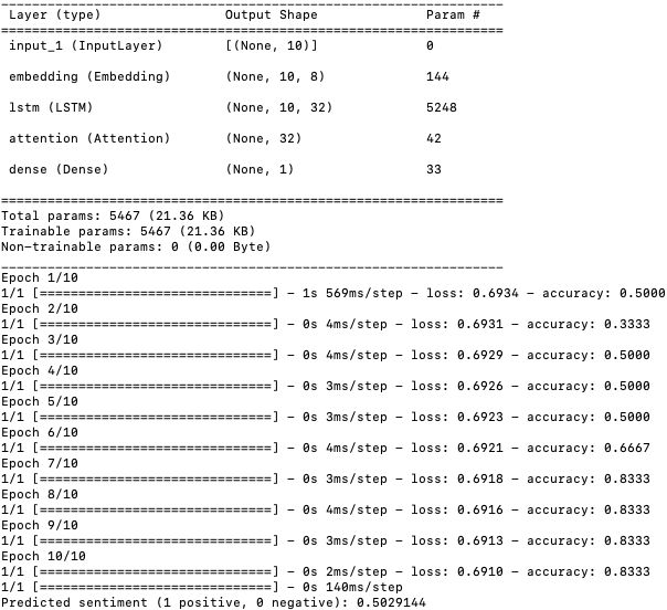
The training accuracy improves as the model progresses through the epochs, which is a good sign that it's learning from the training data.
A few observations and potential improvements are below:

• Training Data Size: The model is trained on a very small dataset (only 6 sentences). This small size might limit the model's ability to generalize well to new, unseen data. If possible, consider using a larger dataset for training.
• Epochs and Overfitting: Although the model's accuracy improves, training on such small data for too many epochs might lead to overfitting.
• Watch for discrepancies between training and validation accuracies with introducing a validation set.
• Model Complexity: The model is relatively simple, which is appropriate given the small dataset. However, if we scale up the data, we might also want to explore more complex architectures or additional features like dropout for regularization.
• Exploring Predictions: Since the predicted sentiment is close to 0.5, it suggests that the model might be somewhat uncertain about the input.
• Adjusting thresholds or further tuning might be necessary to achieve clearer distinctions in predictions.
  

AGNN can also be used for image analysis. However, to adapt the script to handle image analysis, for instance, focusing on identifying defects in complex images such as those from Scanning Electron Microscopy (SEM), we'll need to change several aspects of the model architecture. Instead of a sequence processing model (LSTM), we will switch to a convolutional neural network (CNN), which is more suited for image data. We will also integrate an attention mechanism in a way that aligns with image processing, focusing on periodical structures within SEM images. The code does:

• Use a convolutional base to extract features from SEM images.

  x = Conv2D(32, (3, 3), activation='relu')(inputs)
  x = MaxPooling2D((2, 2))(x)
  x = Conv2D(64, (3, 3), activation='relu')(x)
  x = MaxPooling2D((2, 2))(x)
  x = Conv2D(128, (3, 3), activation='relu')(x)

  Here are what each line does:

  • Conv2D(32, (3, 3), activation='relu')(inputs): This line adds a 2D convolutional layer with 32 filters, each of size 3x3, and a ReLU activation function. This layer is applied directly to the input images and starts the feature extraction by creating 32 feature maps.
  • MaxPooling2D((2, 2))(x): This line applies a 2x2 max pooling operation to the feature maps generated by the previous convolutional layer. Max pooling reduces the spatial dimensions (height and width) of the feature maps, making the model more robust to variations in the position of features in the input images and reducing computational load.
  • Conv2D(64, (3, 3), activation='relu')(x): Adds another convolutional layer with 64 filters of size 3x3, increasing the depth of the network. This layer further processes the reduced feature maps from the previous max pooling layer, extracting more complex features.
  • MaxPooling2D((2, 2))(x): Another max pooling layer that further reduces the spatial dimensions of the feature maps, continuing to condense the information into more abstract representations.
  • Conv2D(128, (3, 3), activation='relu')(x): This final convolutional layer with 128 filters continues to increase the depth and complexity of the feature representations. It’s typically deeper into the network where more abstract and detailed features are learned.
    
• Incorporate a custom attention layer that generates an "attention score" for different regions, indicating potential defects. The line of code that handle the incorporation of the custom attention layer to generate an "attention score" for different regions in the SEM image analysis script is:

  attention_output, attention_weights = ImageAttention()(x)

  Here’s what these specific lines do:

  • Custom Attention Layer Invocation: ImageAttention()(x) creates an instance of the ImageAttention class and passes the output of the previous layer (x) as input. This custom layer is designed to process these inputs and apply the attention mechanism.
  • Attention Output and Weights: The custom attention layer returns two outputs: attention_output and attention_weights.
    • attention_output is the aggregated feature vector after applying the attention weights to the input features, which effectively allows the network to focus on more informative regions of the image.
    • attention_weights represent the "attention score" for different regions of the input feature maps, indicating the significance or relevance of each area for the defect detection task. These scores can be visualized to understand which parts of the image the model is focusing on, potentially pointing to areas with defects.

• Use this score to guide the examination of the images. the specific role of guiding the examination of images using the attention score is primarily conceptualized within the custom ImageAttention layer. This layer computes an attention score and weights that can be used to analyze which parts of the image are most important for the model’s decision-making process. Here's how it's integrated:

  attention_output, attention_weights = ImageAttention()(x)

  In this line, the ImageAttention layer is applied to the feature maps generated by the convolutional layers (x). This operation results in two outputs:

  • attention_output: This is the aggregated feature map after applying the attention weights, which effectively is a summary of the most important features according to the model. It’s used directly for the classification task.
  • attention_weights: These are the actual attention scores for each part of the feature map. This map highlights the regions of the image that the network deems significant in influencing its output.

  The attention weights (attention_weights) are the key element used to guide the examination of the images. These weights can be visualized as a heatmap overlaid on the original image to show which areas are most important. This visualization helps in understanding why the model might be predicting a defect in a specific area of an image, guiding further manual review or automated analysis to focus on these regions.

• Convolutional Layers: These layers are used to process and extract features from the image.
• Global Average Pooling: Reduces each feature map to a single number by taking the average of the values, making the network invariant to the input size.
• Custom Attention Layer: This layer generates a weight map (attention map) that indicates areas of the image that are most relevant for predicting defects. It also combines these features to create a single output vector for the classification layer.
• Attention Mechanism: The core characteristic of an AGNN is its use of an attention mechanism to guide the focus of the neural network. In the modified script, the custom ImageAttention layer serves this purpose by computing attention weights that indicate which regions of the image are more significant for making a decision. This is crucial for tasks like defect detection in SEM images, where not all parts of the image are equally relevant.
• Guided Feature Extraction: The network uses convolutional layers to extract features from the image. The attention weights produced by the ImageAttention layer then guide the network by emphasizing certain features over others. This selective emphasis helps the model focus on potential defect areas.
• Processing Strategy: By incorporating the attention mechanism through a weighted sum of the features (guided by the attention scores), the network effectively focuses its processing on parts of the image identified as potentially problematic. This is in line with the AGNN's goal of focusing neural processing based on relevance to the task at hand.
• Application-Specific Adaptation: The script is tailored to detect defects in periodical structures within SEM images. This specificity is a typical application of AGNNs where the attention mechanism is adapted to the particular characteristics and requirements of the task, such as focusing on minute anomalies in complex patterns.
• Enhance the image areas with high attention scores and apply additional analysis tools to these regions by integrating some post-processing steps into our image processing pipeline.
  • Visualize Attention: This function visualizes the original images alongside their enhanced versions, where the enhancement is based on the attention weights. Each pixel's intensity in the image is scaled by the attention score, making high-attention areas more visible.
  • Further Analysis: This function identifies regions in each image where the attention score exceeds a certain threshold (e.g., 50%). It then isolates these areas for further analysis, which might involve additional diagnostics or processing. The example shows these regions, but in practice, you could integrate more sophisticated image analysis techniques tailored to the specifics of the SEM images or the type of defects being analyzed.

• Encoder: Compresses the image to a lower-dimensional representation.
• Attention Mechanism: Could be integrated in the bottleneck (the compressed feature space) to highlight areas of interest or features critical for detecting defects.
• Decoder: Reconstructs the image, potentially focusing on regions flagged by the attention mechanism.

Such an architecture could help in emphasizing subtle yet crucial discrepancies between the reconstructed and original images, which are indicative of defects. The code shows a simple conceptual sketch of how this might be organized. This hybrid model leverages the autoencoder's ability to reconstruct and the attention mechanism's capacity to highlight significant areas, offering a powerful tool for detailed image analysis tasks like defect detection in complex imaging contexts.

Figure 3300 shows the overall architecture of an Attention-Guided Autoencoder (AGA) using a diagram.

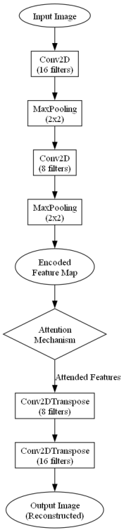
Figure 3300. Overall architecture of an Attention-Guided Autoencoder (code).

===========================================