=================================================================================

Overfitting, underfitting, and the bias-variance tradeoff are foundational concepts that describe the performance of a model in relation to its complexity in machine learning:
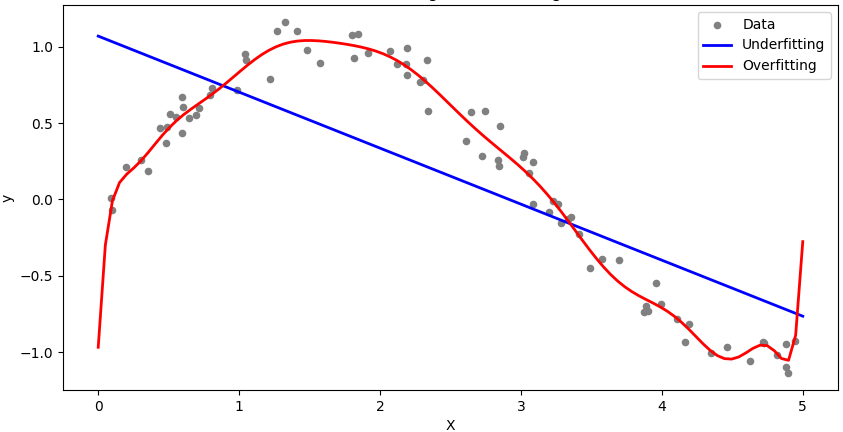
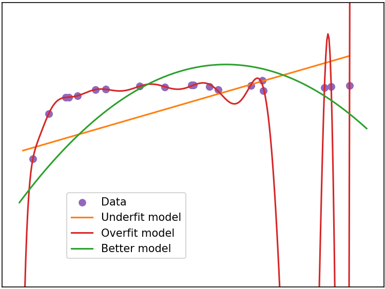
          i) Overfitting. Mathematically, overfitting can be described as a model that has low bias and high variance. The performance on the training data, used to fit the model, is substantially better than performance on a test set. High variance can lead to overfitting. It means the model is too complex and fits the noise in the data rather than the actual patterns. In other words, it fits the training data perfectly but doesn't generalize well to new, unseen data. The reason of overfitting with a model is normally the model has too many parameters or features. For example, a very high-degree polynomial model trying to fit a small dataset.
          ii) Underfitting. Mathematically, underfitting can be described as a model that has high bias and low variance. The model is not fitting the training data very well. It means the model is too simple to capture the underlying patterns in the data. In this case, it has high bias. Namely, high bias can lead to underfitting, where the model is too simplistic and cannot capture the underlying patterns in the data. The reason of underfitting with a model is normally the model has too few parameters or features. For example, a linear model trying to fit highly nonlinear data.

Figure 2379a shows bias-variance trade-off, and underfitting and overfitting in machine learning.

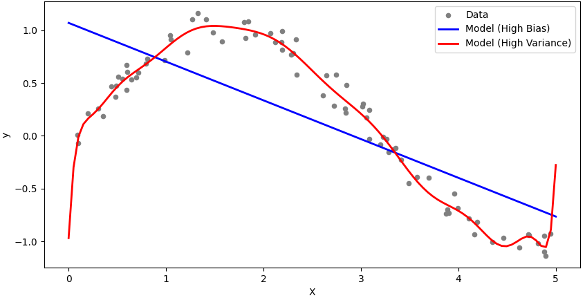
(a)

(b)

To find the right balance between underfitting and overfitting, you typically use techniques like cross-validation and validation datasets to assess model performance. These techniques help you select a model that generalizes well to unseen data and doesn't underfit or overfit.

In addition to this simplified mathematical description, you can also use more complex metrics like learning curves, bias-variance trade-off analysis, or measures like the mean squared error (MSE) to assess the level of underfitting or overfitting in your models.

Figure 2379b shows the training error depending on model complexity. The high degree of polynormial the smaller the training error ideally as shown by the blue curve in Figure 2379b. That is, a higher degree polynomial can potentially fit the training data more closely, resulting in a smaller training error (often measured as mean squared error or a similar metric). This is because a higher degree polynomial can introduce more flexibility and complexity into the model, allowing it to capture intricate patterns and variations in the training data.

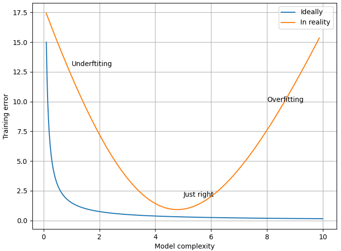
Figure 2379b. Training error versus model complexity (code).

However, in reality, there are important caveats to consider as shown in the orange curve in Figure 2379b:

1. The training error reduces with increase of model complexity at the beginning of increase of model complexity; and then at some model complexity, the error is minimum; however, it increases with further increase of model complexity so that it shows overfitting.

2. Strength of regularization: The strength of regularization is controlled by a hyperparameter, often denoted as λ. When λ is large, it is easier to underfit the data, and when λ is small, which also follows the orange curve in Figure 2379b.

   a. Large λ (Strong Regularization):
• When λ is large, the regularization term dominates the loss function. This means that the model is heavily penalized for having large parameter values.
• Large parameter values can lead to complex and highly flexible models, which are prone to fitting noise in the training data.
• As λ increases, the model becomes more constrained, forcing the parameter values to be small, and effectively simplifying the model.
• This simplification can result in underfitting because the model may not have enough flexibility to capture the underlying patterns in the data. It may generalize poorly both on the training data and new, unseen data.

b. Small λ (Weak Regularization):
• When λ is small, the regularization term has less influence on the loss function, and the model is free to fit the training data more closely.
• Small parameter values may not be penalized as much, allowing the model to have larger, more complex parameter values.
• This can lead to overfitting, where the model becomes too tailored to the training data and captures noise rather than true patterns.
• While the model may perform very well on the training data, it is likely to perform poorly on new, unseen data.
3. Overfitting: While increasing the degree of the polynomial can reduce training error, it can also make the model overly complex and sensitive to noise in the data. This can lead to overfitting, where the model fits the training data extremely well but performs poorly on unseen data. In this case, the model may have a very low training error but a high test (or validation) error, which is undesirable.
4. Computational Complexity: Higher degree polynomials require more parameters, making the model more computationally intensive to train. Additionally, they may require more data to generalize effectively.
5. Occam's Razor: Occam's Razor is a principle in science and machine learning that suggests simpler models are generally preferred over more complex ones when they have similar performance. This is because simpler models are often more interpretable and less prone to overfitting.

============================================

Overfitting and underfitting: code:
          
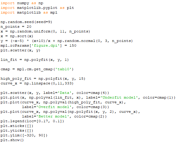
Output: